Current-based LIF
Simulate current-based LIF cells driven by exponential current synapses.
Four independent Poisson spike trains drive 16 current-based leaky integrate-and-fire cells. Each input spike adds synaptic current, which decays exponentially. That current moves the membrane voltage towards threshold; a cell spikes and resets when it crosses threshold. This example shows the input, output spikes, membrane voltage and synaptic current on one shared time axis.
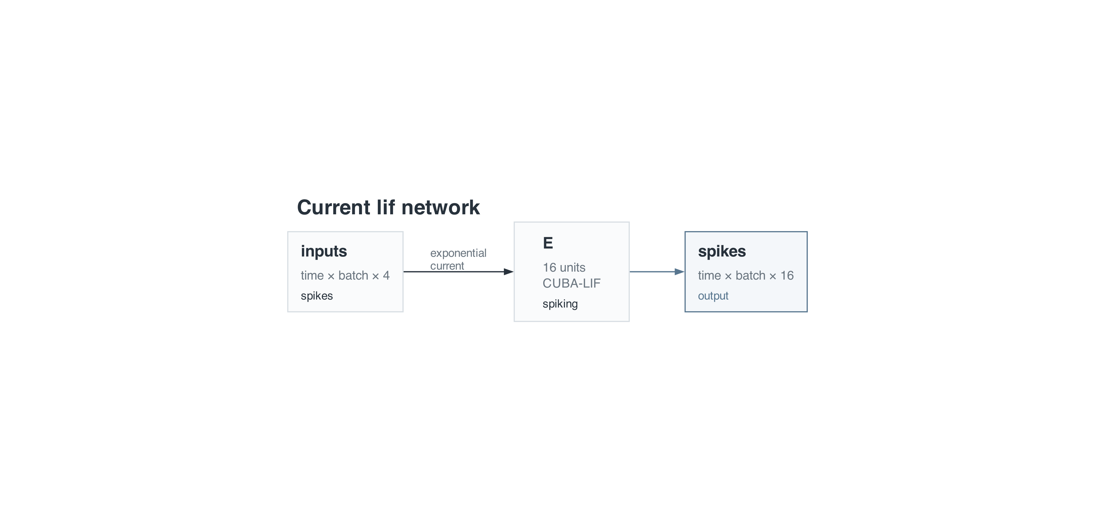
Run from the repository root:
uv run python examples/current-lif/current_lif.pyThe script saves network.png and current-lif.png beside itself. Graphviz’s dot executable is required for the diagram.
1. Imports and network definition
from snnlab import lang, viz
from snnlab.sim.execution import ExecutionSpec, PoissonInputBinding, simulate

DT_MS = 0.5
DURATION_MS = 500
INPUT_RATE_HZ = 80
SEED = 17net = lang.Network("current_lif", dt=DT_MS * lang.ms)2. Define inputs and their binding
inputs = net.input(
    "inputs", shape=("time", "batch", 4), signal_type="spikes", unit="spike"
)
poisson_input = PoissonInputBinding(
    input_id="inputs",
    steps_count=round(DURATION_MS / DT_MS),
    rates_hz=(INPUT_RATE_HZ,),
    seed=SEED,
)
The network input declares four spike channels. The binding supplies 500 ms of Poisson spikes at 80 Hz per channel, using a fixed seed. See ExecutionSpec input bindings for dense arrays/tensors, event streams and dataset inputs.
3. Define the current-based network
cells = net.population(
    "E", size=16, neuron=lang.CUBA_LIF(tau_mem=20 * lang.ms, capacitance_nf=1.0)
)
# Connect all 4 input channels to all 16 E cells using 64 weights.
projection = net.connect(
    inputs,
    cells.excitatory,
    name="input_to_E",
    synapse=lang.ExponentialCurrent(tau=5 * lang.ms),
    weight=lang.Uniform(4.0, 6.0),
    constraint=lang.NonNegative(),
)
CUBA_LIF uses a membrane time constant of 20 ms and capacitance of 1 nF. Its default resting and reset voltages are −65 mV, with threshold at −50 mV. ExponentialCurrent uses a 5 ms decay time constant. Unlike a conductance synapse, this input current does not depend on membrane voltage or a reversal potential.
The all-to-all connection automatically creates a (16, 4) weight matrix: 64 weights, one row per cell and one column per input channel. Uniform(4.0, 6.0) draws initialization values; the executor divides these by the four-channel fan-in, giving initial weights between 1 and 1.5 nA. Each spike adds its weight to the synaptic current. NonNegative keeps these excitatory weights nonnegative.
Current synapses use nA; conductance synapses use uS. The compiler checks compatibility. A projection into cells.inhibitory would subtract its current from the membrane drive.
4. Choose outputs and expose diagnostics
# The official network output: spikes.
net.output("spikes", cells.spikes)
# Expose input spikes and membrane voltage for diagnostics.
net.expose(inputs, name="input_spikes")
net.expose(cells.voltage, name="e_voltage")
net.expose(projection.current, name="e_current")
Spikes are the official output. Inputs, voltage and current are diagnostic signals, returned by default. Use projection.current for current-based synapses.
5. Bundle the network and generate its diagram
bundle = lang.compile(net, target="tools/snnsim")
diagram = lang.diagram(bundle, view="expanded")
viz.render_diagram(
    diagram,
    OUTPUT_DIR / "network.png",
    scale=2,
    height_to_width_ratio=None,
    canvas_size=(1920, 900),
)
The bundle stays in a Python variable here. You can also save it with bundle.write(path) and load it later with lang.load_bundle(path).
6. Configure execution and simulate
execution = ExecutionSpec(
    kind="simulate",
    graph=bundle.graph,
    input_bindings=(poisson_input,),
    seed=SEED,
    device="cpu",
)
result = simulate(execution)
simulate uses the graph executor by default. This example runs on CPU; no training recipe is needed.
7. Retrieve the results
data = result.numpy(batch=0)
input_spikes = data.diagnostics["input_spikes"]
spikes = data.outputs["spikes"]
voltages = data.diagnostics["e_voltage"]
currents = data.diagnostics["e_current"]
time_ms = data.time_ms
assert time_ms is not None
result.numpy(batch=0) converts tensors into NumPy arrays and selects the only batch item. Outputs and diagnostics retain their names, while time_ms supplies the shared time axis. Plotting code is included in the full script below.
8. Full example
"""Simulate current-based LIF cells and plot their input, spikes, voltage and current."""

from pathlib import Path

import matplotlib

matplotlib.use("Agg")
import matplotlib.pyplot as plt
import numpy as np

from snnlab import lang, viz
from snnlab.sim.execution import ExecutionSpec, PoissonInputBinding, simulate

OUTPUT_DIR = Path(__file__).resolve().parent
DT_MS = 0.5
DURATION_MS = 500
INPUT_RATE_HZ = 80
SEED = 17


def main():
    # 1. Create the network.
    net = lang.Network("current_lif", dt=DT_MS * lang.ms)
    # 2. Define the input and its stimulus binding.
    inputs = net.input(
        "inputs", shape=("time", "batch", 4), signal_type="spikes", unit="spike"
    )
    poisson_input = PoissonInputBinding(
        input_id="inputs",
        steps_count=round(DURATION_MS / DT_MS),
        rates_hz=(INPUT_RATE_HZ,),
        seed=SEED,
    )
    # 3. Define the excitatory layer and its input projection.
    cells = net.population(
        "E", size=16, neuron=lang.CUBA_LIF(tau_mem=20 * lang.ms, capacitance_nf=1.0)
    )
    # Connect all 4 input channels to all 16 E cells using 64 weights.
    projection = net.connect(
        inputs,
        cells.excitatory,
        name="input_to_E",
        synapse=lang.ExponentialCurrent(tau=5 * lang.ms),
        weight=lang.Uniform(4.0, 6.0),
        constraint=lang.NonNegative(),
    )
    # 4. Choose outputs and exposed diagnostics.
    # The official network output: spikes.
    net.output("spikes", cells.spikes)
    # Expose input spikes and membrane voltage for diagnostics.
    net.expose(inputs, name="input_spikes")
    net.expose(cells.voltage, name="e_voltage")
    net.expose(projection.current, name="e_current")
    # 5. Compile the network into a bundle.
    bundle = lang.compile(net, target="tools/snnsim")
    diagram = lang.diagram(bundle, view="expanded")
    viz.render_diagram(
        diagram,
        OUTPUT_DIR / "network.png",
        scale=2,
        height_to_width_ratio=None,
        canvas_size=(1920, 900),
    )

    # 6. Describe the execution and simulate.
    execution = ExecutionSpec(
        kind="simulate",
        graph=bundle.graph,
        input_bindings=(poisson_input,),
        seed=SEED,
        device="cpu",
    )
    result = simulate(execution)
    # 7. Retrieve named results and select the first (only) batch item.
    data = result.numpy(batch=0)
    input_spikes = data.diagnostics["input_spikes"]
    spikes = data.outputs["spikes"]
    voltages = data.diagnostics["e_voltage"]
    currents = data.diagnostics["e_current"]
    time_ms = data.time_ms
    assert time_ms is not None

    # Plot the results with snnlab.viz and Matplotlib.
    grid = viz.FigureGrid(
        rows=4, columns=1, bounds=(0.14, 0.07, 0.82, 0.86), row_gap=0.07
    )
    grid.place("inputs", row=0, column=0)
    grid.place("spikes", row=1, column=0)
    grid.place("voltage", row=2, column=0)
    grid.place("current", row=3, column=0)
    figure = grid.figure(figsize=(8, 10), dpi=150)
    input_axis = grid.add_axes(figure, "inputs")
    spike_axis = grid.add_axes(figure, "spikes", sharex=input_axis)
    voltage_axis = grid.add_axes(figure, "voltage", sharex=input_axis)

    current_axis = grid.add_axes(figure, "current", sharex=input_axis)

    for axis, values, title, label in (
        (input_axis, input_spikes, "Input spikes (4 channels)", "Input channel"),
        (spike_axis, spikes, "E spikes (16 cells)", "E cell"),
    ):
        steps, cell_ids = np.nonzero(values)
        axis.scatter(time_ms[steps], cell_ids, marker="|", s=24, color="#1a1a1a")
        axis.set_ylim(-0.5, values.shape[1] - 0.5)
        axis.set_yticks(
            np.linspace(0, values.shape[1] - 1, min(values.shape[1], 4), dtype=int)
        )
        axis.set_ylabel(label)
        axis.set_title(title, pad=10)
        axis.tick_params(labelbottom=False)

    voltage_axis.plot(time_ms, voltages[:, 0], color="#1a1a1a", linewidth=1)
    voltage_axis.set_ylabel("Voltage (mV)")
    voltage_axis.set_title("Membrane voltage of E cell 0", pad=10)
    voltage_axis.tick_params(labelbottom=False)
    current_axis.plot(time_ms, currents[:, 0], color="#1a1a1a", linewidth=1)
    current_axis.set_ylabel("Current (nA)")
    current_axis.set_title("Synaptic current into E cell 0", pad=10)
    current_axis.set_xlabel("Time (ms)")
    voltage_axis.set_xlim(0, DURATION_MS)
    path = OUTPUT_DIR / "current-lif.png"
    figure.savefig(path, bbox_inches="tight")
    plt.close(figure)
    print(f"Saved {path}")

    counts = spikes.sum(axis=0)
    print(f"Total spikes: {int(counts.sum())}")
    print(f"Spikes per cell: {counts.astype(int).tolist()}")


if __name__ == "__main__":
    main()
9. Plots
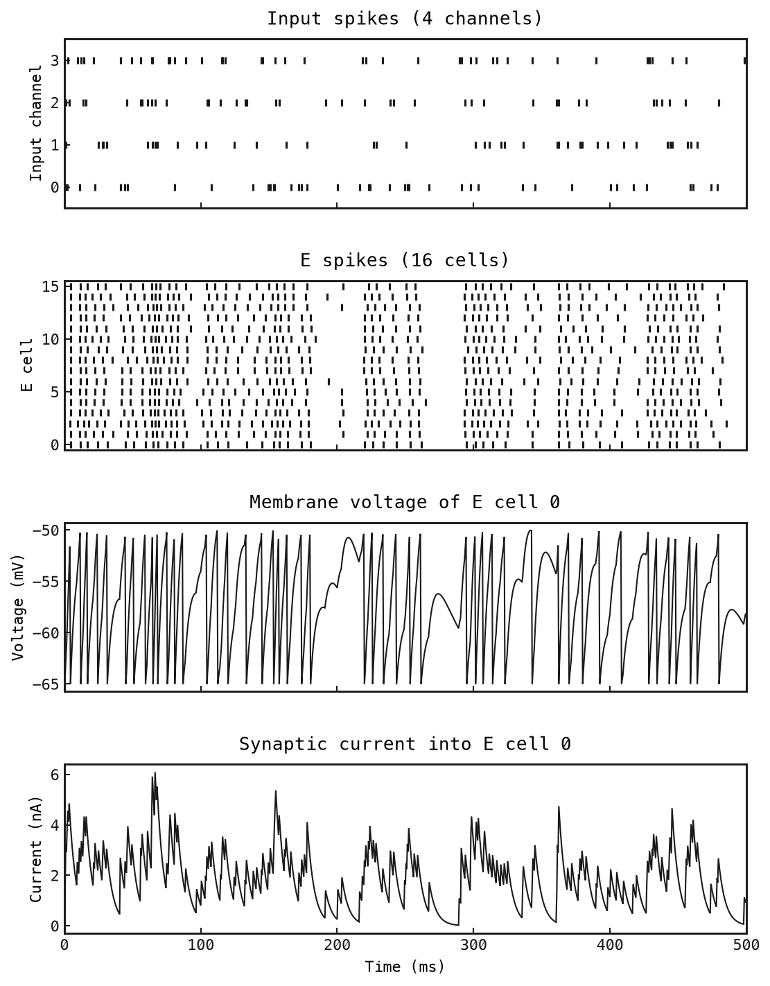
The current rises after input spikes and decays between them. Voltage integrates that drive until threshold crossing resets it. Try reducing INPUT_RATE_HZ or changing the synaptic decay time and compare all four rows.
Continue with Customisation to add spike-triggered adaptation using a registered Python neuron and a custom weight distribution.