Customisation
Compare a built-in current-based LIF neuron with a custom adaptive neuron and weight distribution.
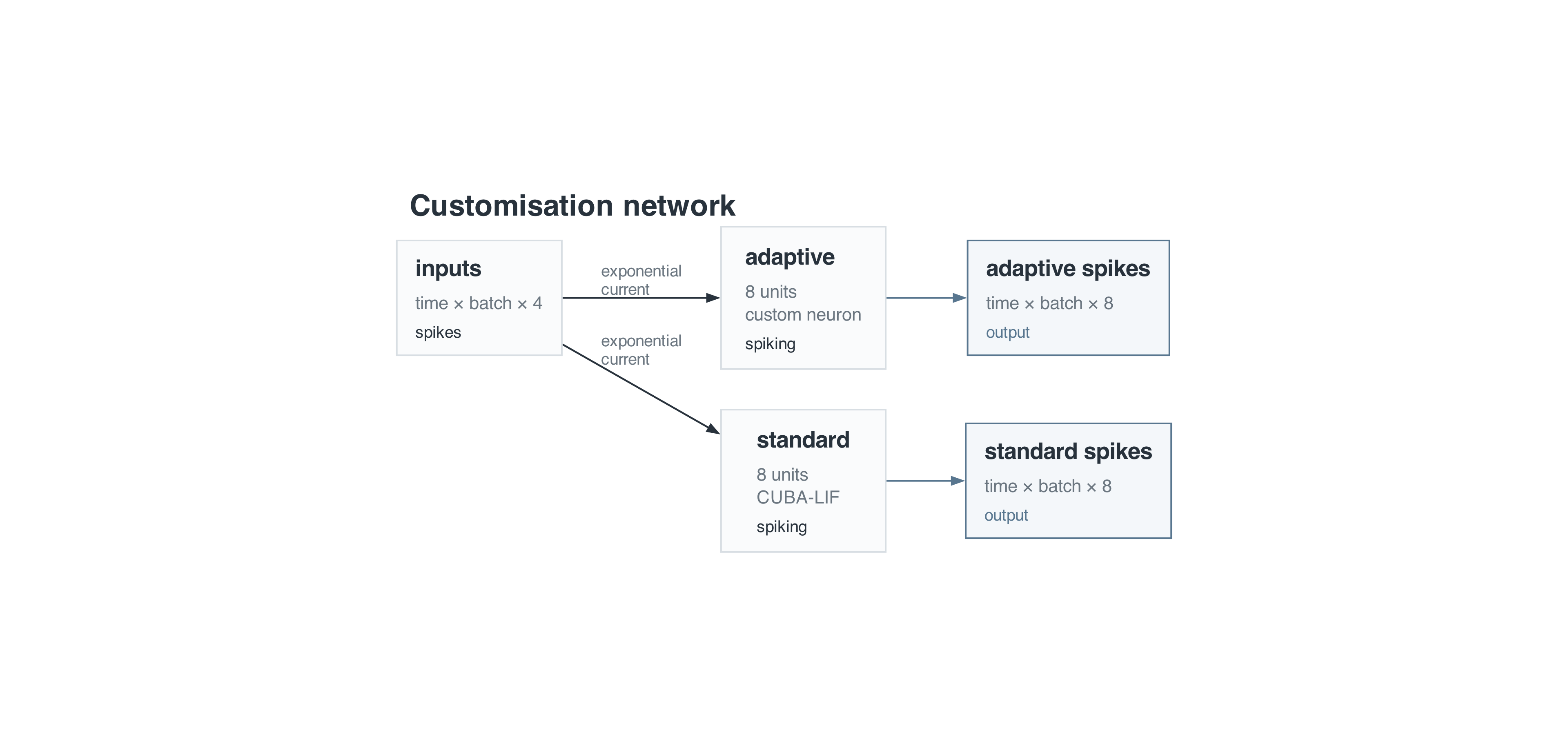
Building on Current-based LIF, this example asks a simple question: how does spike-triggered adaptation change a neuron’s response to sustained input? Four input channels drive two populations of eight cells with exactly the same weights and current-based synapses. One uses the built-in CUBA_LIF; the other uses a registered Python neuron definition that builds an opposing current after each spike.
The stimulus starts at 20 Hz, rises to 120 Hz between 100 and 400 ms, then returns to 20 Hz. The custom population’s adaptation builds up during stimulation and decays afterwards. This is an illustrative discrete-time adaptive model; it is not a claim that one parameterization describes every biological neuron.
Run from the repository root:
uv run python examples/customisation/customisation.pyThe script saves network.bundle, network.png and customisation.png beside itself. Graphviz’s dot executable is needed for the diagram. In a headless environment you can set MPLBACKEND=Agg when running the script.
1. Define the custom neuron
A custom neuron has an initial tensor state and a step function. The step receives previous state, excitatory and inhibitory input, timestep, configuration and a spike function compatible with the run’s surrogate gradient.
def adaptive_initial_state(context):
    shape, device, dtype = context.shape, context.device, context.dtype
    return {
        "voltage": torch.full(shape, -65.0, device=device, dtype=dtype),
        "adaptation": torch.zeros(shape, device=device, dtype=dtype),
    }


def adaptive_step(context):
    voltage = context.state["voltage"]
    adaptation = context.state["adaptation"]
    beta = math.exp(-context.dt_ms / context.config["tau_mem_ms"])
    current = context.excitatory - context.inhibitory - adaptation
    voltage = (
        -65
        + (voltage + 65) * beta
        + current * context.config["tau_mem_ms"] * (1 - beta)
    )
    spikes = context.spike(voltage + 50)
    voltage = torch.where(spikes.bool(), torch.full_like(voltage, -65), voltage)
    adaptation = adaptation * math.exp(-context.dt_ms / context.config["tau_adapt_ms"])
    adaptation = adaptation + spikes * context.config["adaptation_na"]
    return {**context.state, "voltage": voltage, "adaptation": adaptation}, spikes


extensions.register_neuron(
    "example.adaptive_lif/v1",
    adaptive_step,
    initialize=adaptive_initial_state,
    input_unit="nA",
    state_units={"adaptation": "nA"},
)
The initial state provides voltage and adaptation. The executor adds a zero-valued integer refractory tensor when absent. The step returns the updated state and binary spikes. Here adaptation subtracts from the net current and increases by adaptation_na after each spike; its exponential decay is controlled by tau_adapt_ms.
Registration assigns a stable, versioned name. state_units makes adaptation available through population.state("adaptation"). For callback contracts and additional extension categories, see Extensions.
2. Define a custom weight distribution
def clipped_normal(shape, config, *, device, dtype):
    values = torch.randn(shape, device=device, dtype=dtype)
    return (values * config["std"] + config["mean"]).clamp(min=config["minimum"])


extensions.register_initializer("example.clipped_normal/v1", clipped_normal)
The initializer receives the runtime shape, configuration, device and dtype. It draws normal values and clips them at a configurable minimum. Projection initialization subsequently divides by fan-in, and then applies the declared constraint. The name and configuration are stored in the bundle; the Python function remains in the registration module.
See Parameters.
3. Define inputs and the network
net = lang.Network("customisation", dt=DT_MS * lang.ms)
inputs = net.input(
    "inputs", shape=("time", "batch", 4), signal_type="spikes", unit="spike"
)
steps = round(DURATION_MS / DT_MS)
rates = torch.full((steps, 1, 4), 20.0)
rates[round(100 / DT_MS) : round(400 / DT_MS)] = 120.0
generator = torch.Generator().manual_seed(SEED)
input_spikes = (
    torch.rand(rates.shape, generator=generator) < rates * DT_MS / 1000
).float()
binding = DenseArrayBinding("inputs", input_spikes)

# 4. Compare built-in and custom neuron dynamics with matched input weights.
standard = net.population(
    "standard", size=8, neuron=lang.CUBA_LIF(tau_mem=20 * lang.ms)
)
adaptive = net.population(
    "adaptive",
    size=8,
    neuron=lang.CustomNeuron(
        "example.adaptive_lif/v1",
        tau_mem_ms=20,
        tau_adapt_ms=100,
        adaptation_na=0.35,
    ),
)
weights = net.parameter(
    "weights",
    shape=(8, 4),
    unit="nA",
    initializer=lang.CustomInitializer(
        "example.clipped_normal/v1", mean=5.0, std=1.0, minimum=0.0
    ),
    constraint=lang.NonNegative(),
)
for cells in (standard, adaptive):
    projection = net.connect(
        inputs,
        cells.excitatory,
        name=f"input_to_{cells.id}",
        synapse=lang.ExponentialCurrent(tau=5 * lang.ms),
        weight=weights,
    )
    net.output(f"{cells.id}_spikes", cells.spikes)
    net.expose(cells.voltage, name=f"{cells.id}_voltage")
    net.expose(projection.current, name=f"{cells.id}_current")
net.expose(inputs, name="input_spikes")
net.expose(adaptive.state("adaptation"), name="adaptation")
DenseArrayBinding supplies the custom stimulus. The shared parameter has graph shape (8, 4) and unit "nA"; both projections reference it, so differences in response come from neuron dynamics. ExponentialCurrent adds incoming spike-weighted current and lets it decay with a 5 ms time constant. Inhibitory current projections would subtract from membrane drive.
The standard neuron uses the new CUBA_LIF, and the adaptive population uses CustomNeuron. Both expect current input. Mixing these with a conductance synapse is rejected rather than silently interpreting incompatible units.
4. Declare outputs and diagnostics
The loop declares official spike outputs and exposes voltage and synaptic current for both populations. The custom adaptation signal is also exposed. .current belongs to current-based projections; .conductance belongs to conductance-based projections.
Custom state ports participate in normal outputs, diagnostics and operations. Their declared units and (time, batch, cells) axes are preserved in the compiled graph’s signal validation.
5. Compile and simulate
bundle = lang.compile(net, target="tools/snnsim")
bundle.write(OUTPUT_DIR / "network.bundle")
viz.render_diagram(
    lang.diagram(bundle, view="expanded"),
    OUTPUT_DIR / "network.png",
    scale=2,
    height_to_width_ratio=None,
    canvas_size=(1920, 900),
)
execution = ExecutionSpec(
    kind="simulate",
    graph=bundle.graph,
    input_bindings=(binding,),
    seed=SEED,
    device="cpu",
)
result = simulate(execution)
data = result.numpy(batch=0)
assert data.time_ms is not None
The bundle manifest lists required extension names. Import the registration module before loading or executing this bundle in another process. Loading never imports Python code from a bundle. Additional custom state is included in runtime continuation artifacts, so splitting an execution does not reset adaptation or synaptic history.
6. Full example
"""Compare a built-in current LIF with a registered adaptive current neuron.

Run from the repository root: uv run python examples/customisation/customisation.py
Outputs are saved beside this script. Diagram rendering requires Graphviz.
"""

import math
from pathlib import Path

import numpy as np
import torch

from snnlab import extensions, lang, viz
from snnlab.sim.execution import DenseArrayBinding, ExecutionSpec, simulate

OUTPUT_DIR = Path(__file__).resolve().parent
DT_MS = 0.5
DURATION_MS = 500
SEED = 17


# 1. Define a neuron using tensor state and a normal Python step function.
def adaptive_initial_state(context):
    shape, device, dtype = context.shape, context.device, context.dtype
    return {
        "voltage": torch.full(shape, -65.0, device=device, dtype=dtype),
        "adaptation": torch.zeros(shape, device=device, dtype=dtype),
    }


def adaptive_step(context):
    voltage = context.state["voltage"]
    adaptation = context.state["adaptation"]
    beta = math.exp(-context.dt_ms / context.config["tau_mem_ms"])
    current = context.excitatory - context.inhibitory - adaptation
    voltage = (
        -65
        + (voltage + 65) * beta
        + current * context.config["tau_mem_ms"] * (1 - beta)
    )
    spikes = context.spike(voltage + 50)
    voltage = torch.where(spikes.bool(), torch.full_like(voltage, -65), voltage)
    adaptation = adaptation * math.exp(-context.dt_ms / context.config["tau_adapt_ms"])
    adaptation = adaptation + spikes * context.config["adaptation_na"]
    return {**context.state, "voltage": voltage, "adaptation": adaptation}, spikes


extensions.register_neuron(
    "example.adaptive_lif/v1",
    adaptive_step,
    initialize=adaptive_initial_state,
    input_unit="nA",
    state_units={"adaptation": "nA"},
)


# 2. Define an initialization distribution with ordinary PyTorch.
def clipped_normal(shape, config, *, device, dtype):
    values = torch.randn(shape, device=device, dtype=dtype)
    return (values * config["std"] + config["mean"]).clamp(min=config["minimum"])


extensions.register_initializer("example.clipped_normal/v1", clipped_normal)


def main():
    # 3. Define a stimulus with custom tensors: quiet, then sustained activity.
    net = lang.Network("customisation", dt=DT_MS * lang.ms)
    inputs = net.input(
        "inputs", shape=("time", "batch", 4), signal_type="spikes", unit="spike"
    )
    steps = round(DURATION_MS / DT_MS)
    rates = torch.full((steps, 1, 4), 20.0)
    rates[round(100 / DT_MS) : round(400 / DT_MS)] = 120.0
    generator = torch.Generator().manual_seed(SEED)
    input_spikes = (
        torch.rand(rates.shape, generator=generator) < rates * DT_MS / 1000
    ).float()
    binding = DenseArrayBinding("inputs", input_spikes)

    # 4. Compare built-in and custom neuron dynamics with matched input weights.
    standard = net.population(
        "standard", size=8, neuron=lang.CUBA_LIF(tau_mem=20 * lang.ms)
    )
    adaptive = net.population(
        "adaptive",
        size=8,
        neuron=lang.CustomNeuron(
            "example.adaptive_lif/v1",
            tau_mem_ms=20,
            tau_adapt_ms=100,
            adaptation_na=0.35,
        ),
    )
    weights = net.parameter(
        "weights",
        shape=(8, 4),
        unit="nA",
        initializer=lang.CustomInitializer(
            "example.clipped_normal/v1", mean=5.0, std=1.0, minimum=0.0
        ),
        constraint=lang.NonNegative(),
    )
    for cells in (standard, adaptive):
        projection = net.connect(
            inputs,
            cells.excitatory,
            name=f"input_to_{cells.id}",
            synapse=lang.ExponentialCurrent(tau=5 * lang.ms),
            weight=weights,
        )
        net.output(f"{cells.id}_spikes", cells.spikes)
        net.expose(cells.voltage, name=f"{cells.id}_voltage")
        net.expose(projection.current, name=f"{cells.id}_current")
    net.expose(inputs, name="input_spikes")
    net.expose(adaptive.state("adaptation"), name="adaptation")

    # 5. Compile and execute: the bundle stores names/config, not Python code.
    bundle = lang.compile(net, target="tools/snnsim")
    bundle.write(OUTPUT_DIR / "network.bundle")
    viz.render_diagram(
        lang.diagram(bundle, view="expanded"),
        OUTPUT_DIR / "network.png",
        scale=2,
        height_to_width_ratio=None,
        canvas_size=(1920, 900),
    )
    execution = ExecutionSpec(
        kind="simulate",
        graph=bundle.graph,
        input_bindings=(binding,),
        seed=SEED,
        device="cpu",
    )
    result = simulate(execution)
    data = result.numpy(batch=0)
    assert data.time_ms is not None

    # 6. Plot the same stimulus, both responses and the custom adaptation state.
    import matplotlib.pyplot as plt

    layout = viz.FigureGrid(
        rows=4, columns=1, row_gap=0.035, bounds=(0.14, 0.07, 0.82, 0.86)
    )
    for index, name in enumerate(("inputs", "spikes", "voltage", "adaptation")):
        layout.place(name, row=index, column=0)
    figure = layout.figure(figsize=(11, 11))
    axes = [layout.add_axes(figure, "inputs")]
    for name in ("spikes", "voltage", "adaptation"):
        axes.append(layout.add_axes(figure, name, sharex=axes[0]))
    for channel in range(4):
        axes[0].plot(
            data.time_ms[data.diagnostics["input_spikes"][:, channel] > 0],
            np.full(int(data.diagnostics["input_spikes"][:, channel].sum()), channel),
            "|",
            color=viz.Theme().ink,
        )
    axes[0].set_ylabel("Input channel")
    for prefix, offset, color in (
        ("standard", 0, viz.Theme().ink),
        ("adaptive", 9, viz.Theme().accent),
    ):
        spikes = data.outputs[f"{prefix}_spikes"]
        for cell in range(8):
            times = data.time_ms[spikes[:, cell] > 0]
            axes[1].plot(times, np.full(len(times), cell + offset), "|", color=color)
        axes[2].plot(
            data.time_ms,
            data.diagnostics[f"{prefix}_voltage"][:, 0],
            color=color,
            label=prefix,
        )
    axes[1].set_ylabel("Cell")
    axes[1].set_yticks([3.5, 12.5], ["Standard", "Adaptive"])
    axes[2].set_ylabel("Voltage (mV)")
    axes[2].legend(loc="upper right")
    axes[3].plot(
        data.time_ms, data.diagnostics["adaptation"][:, 0], color=viz.Theme().accent
    )
    axes[3].set_ylabel("Adaptation (nA)")
    axes[3].set_xlabel("Time (ms)")
    for axis in axes:
        axis.axvspan(100, 400, color=viz.Theme().rule, alpha=0.5, zorder=-1)
        axis.set_xlim(0, DURATION_MS)
    for axis in axes[:-1]:
        axis.tick_params(labelbottom=False)
    figure.savefig(OUTPUT_DIR / "customisation.png", dpi=160)
    plt.close(figure)
    for prefix in ("standard", "adaptive"):
        print(f"{prefix}: {int(data.outputs[f'{prefix}_spikes'].sum())} spikes")
    print(f"Saved {OUTPUT_DIR / 'customisation.png'}")


if __name__ == "__main__":
    main()
7. Plots
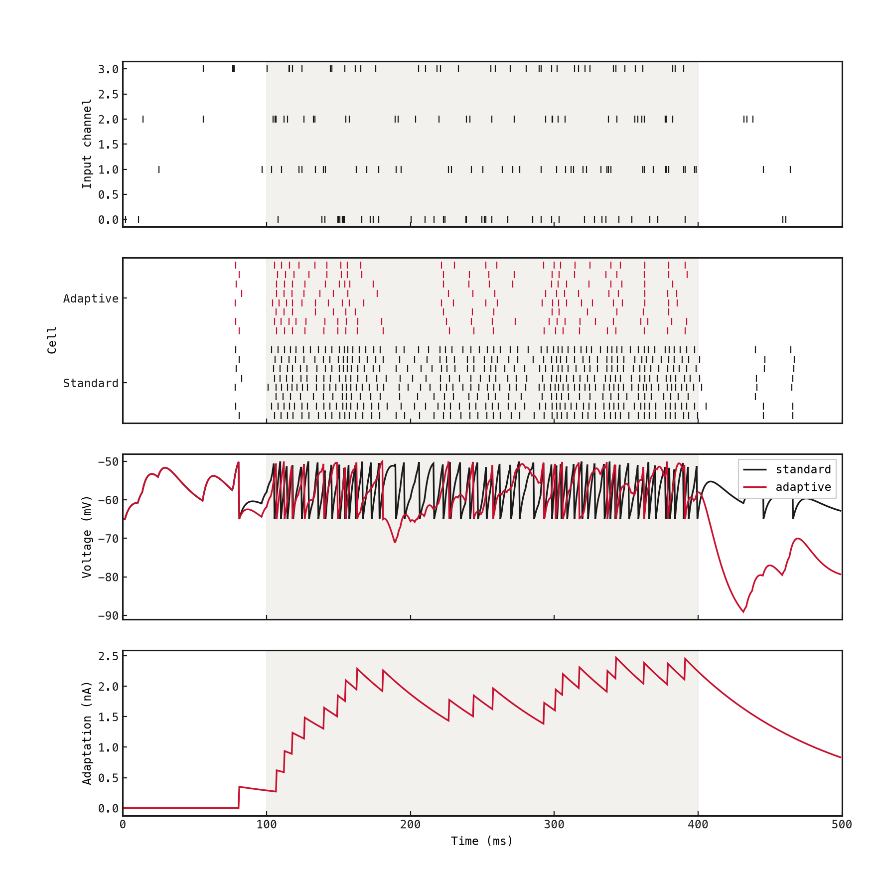
With the supplied seed, the standard population produces 469 spikes and the adaptive population 177. The shaded region marks the increased input rate. Set adaptation_na=0 and rerun: with these matched weights and zero refractory periods, both populations should produce the same response. Then vary the adaptation decay to examine recovery after the stimulus.