Training
Train a spike-pattern classifier, plot loss and accuracy per epoch, and save weights for inference.
Teach the network to recognise which pair of input channels is more active. Each example is a short burst of spikes across four channels. In class A, channels 0 and 1 fire frequently and channels 2 and 3 fire less often; in class B, the pattern is reversed. The exact spikes change from sample to sample, so the network must learn the pattern rather than memorise one spike train.
The network passes these inputs through 16 excitatory neurons into two readout cells, one for each class. Its prediction is the class with the higher score. During training, it compares that prediction with the correct label and adjusts both connections to make future predictions better. Separate validation examples check whether it recognises spike patterns it has not trained on.
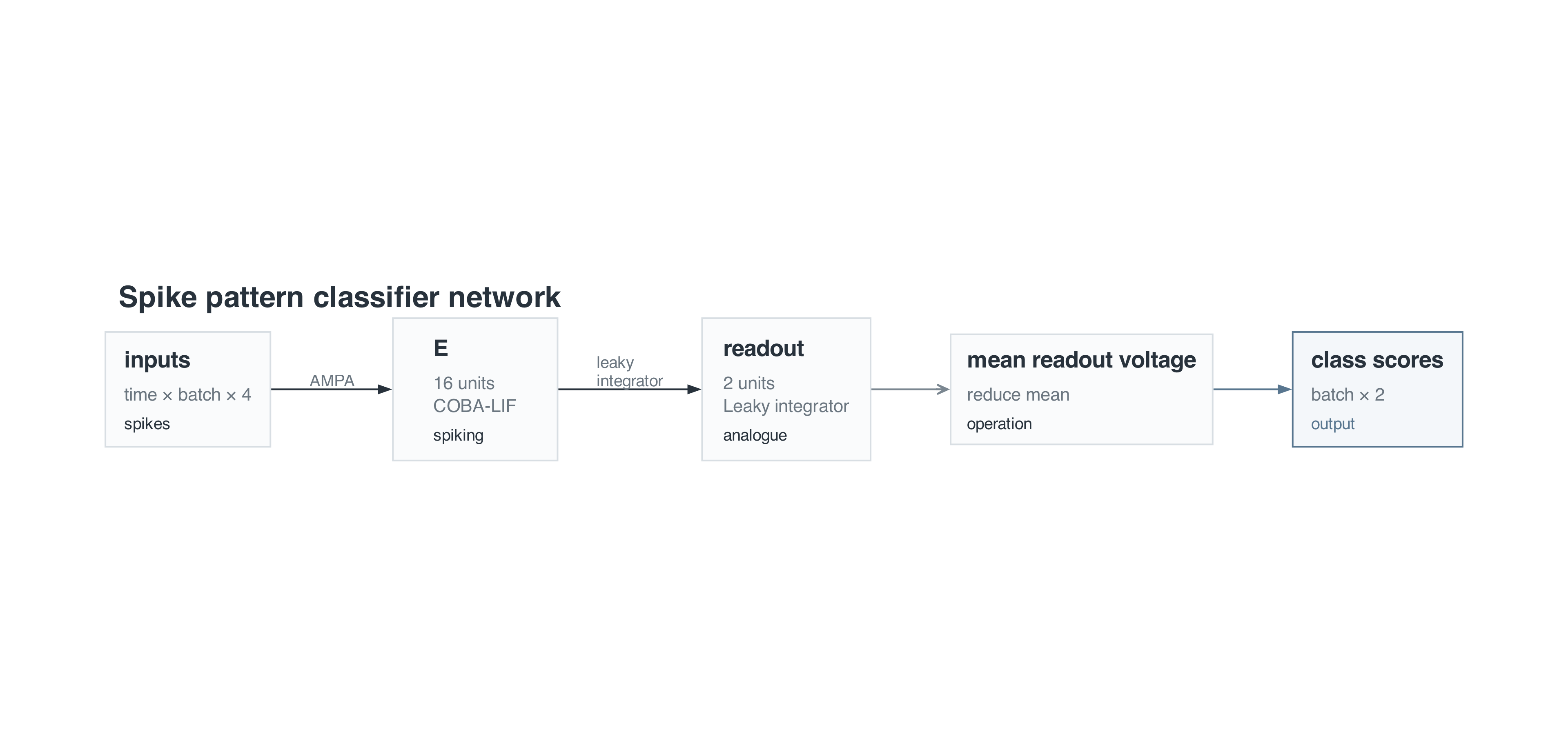
Both the input-to-E weights (w_in) and E-to-readout weights (w_out) learn. Surrogate gradients carry the loss backward through the E neurons’ spikes. The curves below show loss and accuracy after each epoch.
This extends Quickstart with labelled data, minibatches, validation and saved weights. No dataset download is needed. All files live in examples/training/; the saved model can later be reused from the Inference example.
1. Imports and network definition
import json
from pathlib import Path

import numpy as np
import torch

from snnlab import lang, viz
from snnlab.lang import training
from snnlab.sim.execution import (
    DenseArrayBinding,
    ExecutionSpec,
    ValidationSpec,
    save_training_checkpoint,
    train,
)

OUTPUT_DIR = Path(__file__).resolve().parent
DT_MS = 0.5
DURATION_MS = 200
HIGH_RATE_HZ = 100
LOW_RATE_HZ = 10
TRAIN_SAMPLES = 128
VALIDATION_SAMPLES = 64
BATCH_SIZE = 32
EPOCHS = 20
INPUT_LEARNING_RATE = 0.001
READOUT_LEARNING_RATE = 1.0
SEED = 17net = lang.Network("spike_pattern_classifier", dt=DT_MS * lang.ms)Each presentation lasts 200 ms, sampled in 0.5 ms steps. The execution seed fixes initialization and the shuffled training order.
2. Define inputs, labels and bindings
The dataset helper makes balanced classes. Class A has nominal rates [100, 100, 10, 10] Hz and class B has [10, 10, 100, 100] Hz. Each sample receives independent rate variation of ±15% and independent Bernoulli-discretized Poisson spikes.
def make_dataset(samples, seed):
    """Balanced classes with independent rate variation and Poisson spike draws."""
    rng = np.random.default_rng(seed)
    labels = np.arange(samples) % 2
    rng.shuffle(labels)
    patterns = np.array(
        [
            [HIGH_RATE_HZ, HIGH_RATE_HZ, LOW_RATE_HZ, LOW_RATE_HZ],
            [LOW_RATE_HZ, LOW_RATE_HZ, HIGH_RATE_HZ, HIGH_RATE_HZ],
        ]
    )
    rates = patterns[labels] * rng.uniform(0.85, 1.15, size=(samples, 4))
    probability = rates * DT_MS / 1000
    steps = round(DURATION_MS / DT_MS)
    spikes = rng.random((steps, samples, 4)) < probability
    return torch.tensor(spikes, dtype=torch.float32), torch.tensor(
        labels, dtype=torch.long
)inputs = net.input(
"inputs", shape=("time", "batch", 4), signal_type="spikes", unit="spike"
)
train_spikes, train_labels = make_dataset(TRAIN_SAMPLES, seed=SEED + 1)
validation_spikes, validation_labels = make_dataset(
VALIDATION_SAMPLES, seed=SEED + 2
)
train_input = DenseArrayBinding(input_id="inputs", value=train_spikes)
validation_input = DenseArrayBinding(input_id="inputs", value=validation_spikes)Input tensors have (400, samples, 4) axes: time, sample/batch and input channel. Labels are integer class IDs 0 or 1. Training and validation use different random seeds and share no samples.
DenseArrayBinding supplies these custom spike tensors. The training label vector is supplied separately through ExecutionSpec.targets, under the name used by the loss.
3. Define the network and readout
cells = net.population("E", size=16, neuron=lang.COBA_LIF(tau_mem=20 * lang.ms))
input_projection = net.connect(
inputs,
cells.excitatory,
name="input_to_E",
synapse=lang.AMPA(tau=2 * lang.ms),
weight=lang.Uniform(0.0, 0.8),
constraint=lang.NonNegative(),
)
w_in = input_projection.weight
# Two non-spiking readout cells, one per class.
readout = net.population(
"readout",
size=2,
neuron=lang.LeakyIntegrator(tau=20 * lang.ms, initial_voltage=0.0),
spiking=False,
)
# Explicit output weights: 2 readout cells receive spikes from 16 E cells.
w_out = net.parameter(
"w_out", shape=(2, 16), unit="uS", initializer=lang.Normal(0.0, 0.1)
)
net.connect(
cells.spikes,
readout.excitatory,
name="E_to_readout",
synapse=lang.LeakyIntegrator(tau=20 * lang.ms),
weight=w_out,
)
scores = lang.ops.reduce(
readout.voltage, operation="mean", over="time", name="mean_readout_voltage"
)net.connect automatically creates 64 input-to-E weights, with compiled shape (16, 4). w_in = input_projection.weight names the reference to these automatically created weights. They start with a uniform initialization and learn during training, while remaining non-negative. Their initialization is divided by the four input channels at execution, as described in the weight reference.
The readout is an explicit population of two non-spiking leaky-integrator cells, one per class. E_to_readout connects all 16 E cells to both readout cells.
w_out is explicitly declared with shape (2, 16): 32 output weights, one row per readout cell and one column per E cell. It starts with small normally distributed values and is passed to net.connect as weight=w_out. The executor divides projection weights by the source count (16 here). These classifier weights have no non-negative constraint, so learning can make them positive or negative; the input-to-E conductance weights remain non-negative.
Each readout cell integrates its weighted E spikes without emitting spikes. lang.ops.reduce averages the readout voltage over time to produce two class scores per sample, with shape (batch, 2). Cross-entropy treats these scores as logits, rather than probabilities.
This trains both connections: the E layer learns spike features through w_in, and the readout learns how to combine them through w_out. The neuron time constants and other neuron settings remain fixed.
4. Choose outputs and expose diagnostics
net.output("class_scores", scores)
net.expose(inputs, name="input_spikes")
net.expose(cells.spikes, name="e_spikes")
net.expose(readout.voltage, name="readout_voltage")The official output is result.outputs["class_scores"]. Inputs, E spikes and readout voltages are exposed for optional diagnostic inspection. Training and evaluation use diagnostics=False to avoid storing these traces while measuring the learning curves.
5. Define the training recipe
See the Training API reference for objectives, parameter groups, optimizer settings and surrogate gradients.
objective = training.CrossEntropy(prediction=scores, target="class")
readout_parameters = training.ParameterGroup(
(w_out,), name="readout", lr=READOUT_LEARNING_RATE
)
input_parameters = training.ParameterGroup(
(w_in,), name="input_to_E", lr=INPUT_LEARNING_RATE
)
recipe = lang.TrainSpec(
objectives=(objective,),
parameter_groups=(input_parameters, readout_parameters),
optimizer=training.AdamW(weight_decay=0.0),
surrogate=training.FastSigmoid(slope=1.0),
gradient_clip=1.0,
presentation_duration=DURATION_MS * lang.ms,
)CrossEntropy associates the class scores with a target named "class". Its labels must be integers in the range 0 to 1. The two parameter groups select (w_in,) and (w_out,). Their learning rates are INPUT_LEARNING_RATE and READOUT_LEARNING_RATE; the smaller input rate limits changes to the E neurons’ conductances. Neither group is frozen. Every parameter belongs to exactly one group.
training.FastSigmoid(slope=1.0) explicitly enables the fast-sigmoid surrogate for the E neurons. The forward pass still emits discrete spikes; the backward pass uses a smooth approximation to the threshold derivative so gradients reach w_in. Small nonzero initial w_out values allow this gradient path to carry a signal from the first update. gradient_clip=1.0 caps the combined gradient norm before the optimizer step.
AdamW(weight_decay=0.0) updates both connections. TrainSpec declares the loss and optimization rules. The direct ExecutionSpec fields below determine the epoch and minibatch schedule.
6. Bundle the network and recipe
bundle = lang.compile(net, training=recipe, target="tools/snnsim")
diagram = lang.diagram(bundle, view="expanded")
viz.render_diagram(
diagram,
OUTPUT_DIR / "network.png",
scale=2,
height_to_width_ratio=None,
canvas_size=(1920, 900),
)
bundle_path = bundle.write(OUTPUT_DIR / "network.bundle")
checkpoint_path = OUTPUT_DIR / "trained.checkpoint"Compilation validates both the graph and training recipe. network.bundle contains the model structure, initialization and recipe; it does not contain learned weights. The separate trained.checkpoint directory will contain those weights, optimizer state and resume coordinates.
7. Train and evaluate in one call
ValidationSpec supplies held-out input bindings and labels. Pass it to ExecutionSpec.validation, then call train once:
validation = ValidationSpec(
input_bindings=(validation_input,),
targets={"class": validation_labels},
)
execution = ExecutionSpec(
kind="train",
bundle=bundle_path,
input_bindings=(train_input,),
targets={"class": train_labels},
validation=validation,
seed=SEED,
device="cpu",
diagnostics=False,
epochs=EPOCHS,
batch_size=BATCH_SIZE,
shuffle=True,
)
result = train(execution)
assert result.training_checkpoint is not None
save_training_checkpoint(checkpoint_path, result.training_checkpoint)
history = result.metrics["epochs"]
for row in history:
print(
f"Epoch {row['epoch']:02d}: train loss={row['train_loss']:.3f}, "
f"validation loss={row['validation_loss']:.3f}, "
f"train accuracy={row['train_accuracy']:.1%}, "
f"validation accuracy={row['validation_accuracy']:.1%}",
)train handles all 20 epochs internally. Each epoch processes four minibatches of 32 training samples, with shuffle=True changing their order each epoch. Validation samples are evaluated without gradients or optimizer updates.
result.metrics["epochs"] contains loss and accuracy measured after each epoch on the whole training and validation split, plus epoch 0 before learning. These are evaluations of fixed weights, not the last minibatch’s loss or an average collected while weights were changing. Accuracy is the fraction of samples whose highest-scoring class matches the label.
The final checkpoint is saved once for later inference. There is no external epoch loop or intermediate checkpoint management.
8. Save metrics and plot curves
metrics_path = OUTPUT_DIR / "metrics.json"
metrics_path.write_text(json.dumps(history, indent=2) + "\n")metrics.json contains one row per epoch, with training and validation loss and accuracy. Accuracy values are fractions from 0 to 1; the figure displays percentages.
The plotting code makes one two-row figure with a shared epoch axis: cross-entropy above and accuracy below. It is included only in the full example.
9. Full example
Save the complete script as examples/training/training.py. In a repository checkout it is already there.
uv run python examples/training/training.pyIt saves these files beside the script, regardless of the working directory:
network.bundle/: compiled graph and training recipe.trained.checkpoint/: final learned weights, optimizer state and resume coordinates.metrics.json: training and validation measurements for epochs 0–20.training.png: loss and accuracy curves.network.png: diagram generated from the compiled network.
Rendering the network diagram requires Graphviz’s dot executable on your PATH; on macOS, install it with brew install graphviz.
Rerunning starts training from scratch and replaces those generated outputs. It does not automatically resume an earlier run. The Inference example loads examples/training/network.bundle and examples/training/trained.checkpoint, rather than creating new weights or retraining.
"""Train a spike-pattern classifier and save weights and epoch curves beside it."""
import json
from pathlib import Path
import matplotlib
matplotlib.use("Agg")
import matplotlib.pyplot as plt
import numpy as np
import torch
from snnlab import lang, viz
from snnlab.lang import training
from snnlab.sim.execution import (
DenseArrayBinding,
ExecutionSpec,
ValidationSpec,
save_training_checkpoint,
train,
)
OUTPUT_DIR = Path(__file__).resolve().parent
DT_MS = 0.5
DURATION_MS = 200
HIGH_RATE_HZ = 100
LOW_RATE_HZ = 10
TRAIN_SAMPLES = 128
VALIDATION_SAMPLES = 64
BATCH_SIZE = 32
EPOCHS = 20
INPUT_LEARNING_RATE = 0.001
READOUT_LEARNING_RATE = 1.0
SEED = 17
def make_dataset(samples, seed):
"""Balanced classes with independent rate variation and Poisson spike draws."""
rng = np.random.default_rng(seed)
labels = np.arange(samples) % 2
rng.shuffle(labels)
patterns = np.array(
[
[HIGH_RATE_HZ, HIGH_RATE_HZ, LOW_RATE_HZ, LOW_RATE_HZ],
[LOW_RATE_HZ, LOW_RATE_HZ, HIGH_RATE_HZ, HIGH_RATE_HZ],
]
)
rates = patterns[labels] * rng.uniform(0.85, 1.15, size=(samples, 4))
probability = rates * DT_MS / 1000
steps = round(DURATION_MS / DT_MS)
spikes = rng.random((steps, samples, 4)) < probability
return torch.tensor(spikes, dtype=torch.float32), torch.tensor(
labels, dtype=torch.long
)
def main():
# 1. Create the network.
net = lang.Network("spike_pattern_classifier", dt=DT_MS * lang.ms)
# 2. Define inputs, labelled datasets and bindings.
inputs = net.input(
    "inputs", shape=("time", "batch", 4), signal_type="spikes", unit="spike"
)
train_spikes, train_labels = make_dataset(TRAIN_SAMPLES, seed=SEED + 1)
validation_spikes, validation_labels = make_dataset(
    VALIDATION_SAMPLES, seed=SEED + 2
)
train_input = DenseArrayBinding(input_id="inputs", value=train_spikes)
validation_input = DenseArrayBinding(input_id="inputs", value=validation_spikes)
# 3. Define the excitatory layer and two-class readout.
cells = net.population("E", size=16, neuron=lang.COBA_LIF(tau_mem=20 * lang.ms))
input_projection = net.connect(
    inputs,
    cells.excitatory,
    name="input_to_E",
    synapse=lang.AMPA(tau=2 * lang.ms),
    weight=lang.Uniform(0.0, 0.8),
    constraint=lang.NonNegative(),
)
w_in = input_projection.weight
# Two non-spiking readout cells, one per class.
readout = net.population(
    "readout",
    size=2,
    neuron=lang.LeakyIntegrator(tau=20 * lang.ms, initial_voltage=0.0),
    spiking=False,
)
# Explicit output weights: 2 readout cells receive spikes from 16 E cells.
w_out = net.parameter(
    "w_out", shape=(2, 16), unit="uS", initializer=lang.Normal(0.0, 0.1)
)
net.connect(
    cells.spikes,
    readout.excitatory,
    name="E_to_readout",
    synapse=lang.LeakyIntegrator(tau=20 * lang.ms),
    weight=w_out,
)
scores = lang.ops.reduce(
    readout.voltage, operation="mean", over="time", name="mean_readout_voltage"
)
# 4. Declare the official output and optional diagnostics.
net.output("class_scores", scores)
net.expose(inputs, name="input_spikes")
net.expose(cells.spikes, name="e_spikes")
net.expose(readout.voltage, name="readout_voltage")
# 5. Define the loss, trainable parameters and optimizer.
objective = training.CrossEntropy(prediction=scores, target="class")
readout_parameters = training.ParameterGroup(
    (w_out,), name="readout", lr=READOUT_LEARNING_RATE
)
input_parameters = training.ParameterGroup(
    (w_in,), name="input_to_E", lr=INPUT_LEARNING_RATE
)
recipe = lang.TrainSpec(
    objectives=(objective,),
    parameter_groups=(input_parameters, readout_parameters),
    optimizer=training.AdamW(weight_decay=0.0),
    surrogate=training.FastSigmoid(slope=1.0),
    gradient_clip=1.0,
    presentation_duration=DURATION_MS * lang.ms,
)
# 6. Compile and save the bundle for training and later inference.
bundle = lang.compile(net, training=recipe, target="tools/snnsim")
diagram = lang.diagram(bundle, view="expanded")
viz.render_diagram(
    diagram,
    OUTPUT_DIR / "network.png",
    scale=2,
    height_to_width_ratio=None,
    canvas_size=(1920, 900),
)
bundle_path = bundle.write(OUTPUT_DIR / "network.bundle")
checkpoint_path = OUTPUT_DIR / "trained.checkpoint"
# 7. Train and measure each epoch in one call.
validation = ValidationSpec(
    input_bindings=(validation_input,),
    targets={"class": validation_labels},
)
execution = ExecutionSpec(
    kind="train",
    bundle=bundle_path,
    input_bindings=(train_input,),
    targets={"class": train_labels},
    validation=validation,
    seed=SEED,
    device="cpu",
    diagnostics=False,
    epochs=EPOCHS,
    batch_size=BATCH_SIZE,
    shuffle=True,
)
result = train(execution)
assert result.training_checkpoint is not None
save_training_checkpoint(checkpoint_path, result.training_checkpoint)
history = result.metrics["epochs"]
for row in history:
    print(
        f"Epoch {row['epoch']:02d}: train loss={row['train_loss']:.3f}, "
        f"validation loss={row['validation_loss']:.3f}, "
        f"train accuracy={row['train_accuracy']:.1%}, "
        f"validation accuracy={row['validation_accuracy']:.1%}",
    )
# 8. Save epoch metrics and plot training curves.
metrics_path = OUTPUT_DIR / "metrics.json"
metrics_path.write_text(json.dumps(history, indent=2) + "\n")
# Plot the epoch curves.
grid = viz.FigureGrid(
rows=2, columns=1, bounds=(0.13, 0.1, 0.83, 0.82), row_gap=0.09
)
grid.place("loss", row=0, column=0)
grid.place("accuracy", row=1, column=0)
figure = grid.figure(figsize=(8, 6.5), dpi=150)
loss_axis = grid.add_axes(figure, "loss")
accuracy_axis = grid.add_axes(figure, "accuracy", sharex=loss_axis)
epochs = [row["epoch"] for row in history]
for split, color in (("train", "#1a1a1a"), ("validation", "#a74727")):
loss_axis.plot(
epochs,
[row[f"{split}_loss"] for row in history],
label=split.capitalize(),
color=color,
)
accuracy_axis.plot(
epochs,
[100 * row[f"{split}_accuracy"] for row in history],
label=split.capitalize(),
color=color,
)
loss_axis.set_title("Classification loss", pad=10)
loss_axis.set_ylabel("Cross-entropy")
loss_axis.tick_params(labelbottom=False)
loss_axis.legend(frameon=False)
accuracy_axis.axhline(50, color="#888888", linestyle=":", label="Chance (50%)")
accuracy_axis.set_title("Classification accuracy", pad=10)
accuracy_axis.set_ylabel("Accuracy (%)")
accuracy_axis.set_xlabel("Epoch")
accuracy_axis.set_ylim(0, 105)
accuracy_axis.set_xlim(0, EPOCHS)
accuracy_axis.set_xticks(range(0, EPOCHS + 1, 5))
accuracy_axis.legend(frameon=False, loc="lower right")
figure_path = OUTPUT_DIR / "training.png"
figure.savefig(figure_path, bbox_inches="tight")
plt.close(figure)
print(f"Saved {figure_path}")
print(f"Saved {metrics_path}")
print(f"Inference can load {bundle_path} and {checkpoint_path}")
if __name__ == "__main__":
main()10. Training curves
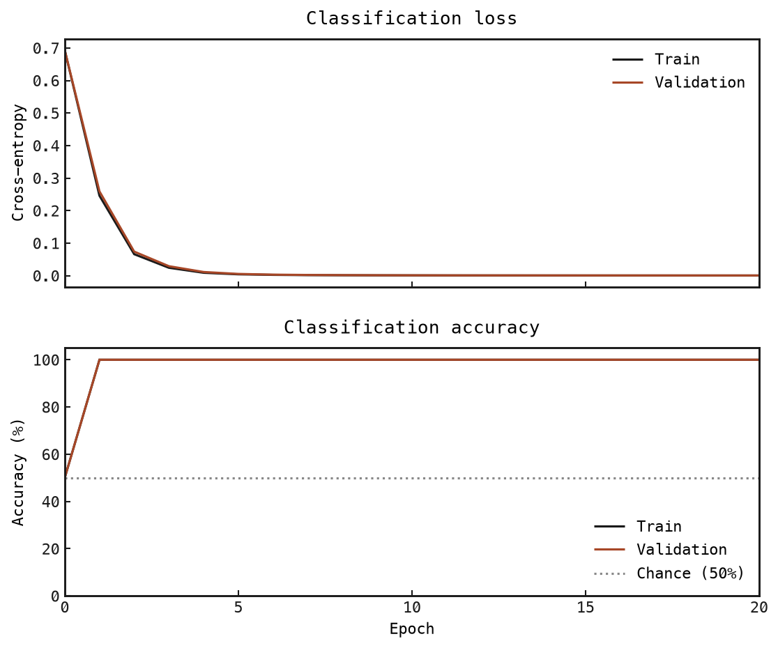
With the supplied seeds, both accuracies rise from 50% at epoch 0 to 100% after the first epoch, while cross-entropy continues to decrease. This is deliberately an easy classification problem.
The held-out validation curve measures this synthetic task, not generalization to real neural recordings. A gap between training and validation accuracy indicates that training performance alone overstates performance on unseen samples.
Change EPOCHS, INPUT_LEARNING_RATE or READOUT_LEARNING_RATE, rerun, and compare the curves while keeping the data seeds fixed.