PyTorch Integration
Reuse a saved snnlab network inside a PyTorch module and train it with your own data loaders, loss, optimizer and epoch loop.
Combine snnlab’s spiking network with ordinary PyTorch layers in one trainable model. This example reuses examples/training/network.bundle and trains fresh weights for the same task: recognise which pair of four input channels is more active.
The saved bundle supplies the spiking architecture, trainable parameter names, learning rates, constraints and surrogate configuration. Its two output values feed an external Linear(2, 8) → ReLU → Linear(8, 2) head, defined with ordinary PyTorch modules. PyTorch handles batching, loss calculation, backpropagation, optimizer steps, evaluation and saving weights. There are no calls to snnlab.sim.execution.train, simulate or infer.
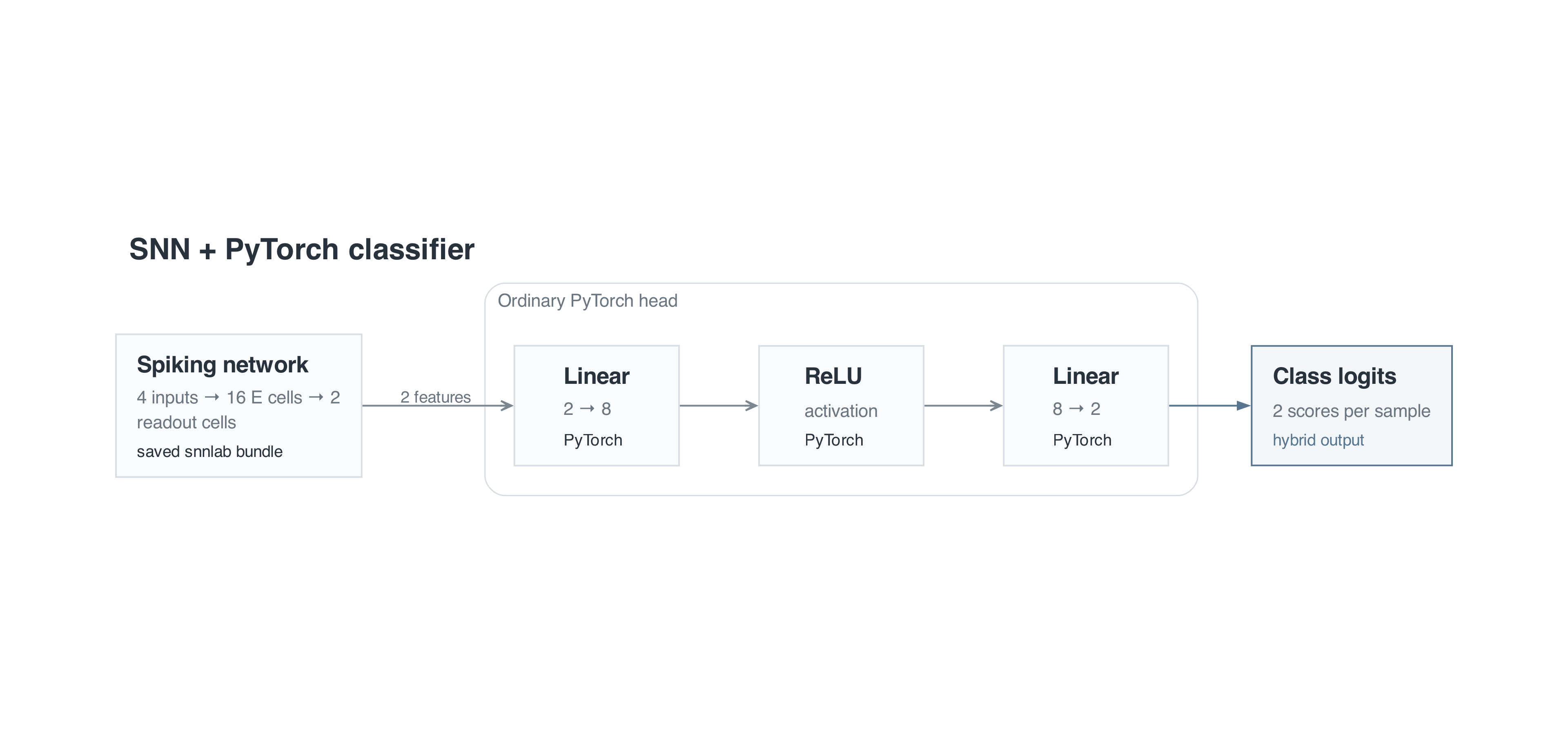
Unlike Inference, this example does not load Training’s trained.checkpoint. It starts a new training run using the same architecture and initialization rules. Its outputs live separately in examples/pytorch/.
1. Load the bundle
import json
from pathlib import Path

import numpy as np
import torch
from torch import nn
from torch.utils.data import DataLoader, TensorDataset

from snnlab import lang, viz
from snnlab.sim.execution import GraphExecutor, plan_graph

OUTPUT_DIR = Path(__file__).resolve().parent
TRAINING_DIR = OUTPUT_DIR.parent / "training"
DEVICE = "cpu"
SEED = 17
EPOCHS = 20
BATCH_SIZE = 32
HEAD_LEARNING_RATE = 0.01
DT_MS = 0.5
DURATION_MS = 200
TRAIN_SAMPLES = 128
VALIDATION_SAMPLES = 64
TEST_SAMPLES = 64bundle_path = TRAINING_DIR / "network.bundle"
if not bundle_path.is_dir():
raise FileNotFoundError(
f"Missing {bundle_path}. Run uv run python examples/training/training.py first."
)
bundle = lang.load_bundle(bundle_path)
recipe = bundle.training
if recipe is None:
raise ValueError("Run Training to generate a bundle with a training recipe.")Run Training first to generate the bundle. lang.load_bundle verifies and loads the saved graph and recipe. It does not compile a new network or load learned weights. The full script generates the hybrid diagram from the saved graph and the actual head modules. Diagram rendering requires Graphviz’s dot executable on your PATH.
2. Combine the SNN with ordinary PyTorch layers
See the GraphExecutor API reference for construction, tensor shapes and live parameter access.
GraphExecutor already subclasses torch.nn.Module. plan_graph prepares the compiled graph for execution. The wrapper below adapts batch-first tensors, runs the SNN, then passes its output through a separate nn.Sequential head:
class Classifier(nn.Module):
"""Compose the bundled SNN with an ordinary PyTorch classification head."""
def __init__(self, bundle):
super().__init__()
recipe = bundle.training
if recipe is None:
raise ValueError("The saved bundle must include its training recipe.")
self.snn = GraphExecutor(
plan_graph(bundle.graph),
seed=SEED,
trainable_parameters=recipe["resolved_parameters"]["trainable"],
surrogate_slope=float(recipe["surrogate"]["slope"]),
)
self.head = nn.Sequential(
nn.Linear(2, 8),
nn.ReLU(),
nn.Linear(8, 2),
)
def forward(self, spikes):
result = self.snn({"inputs": spikes.transpose(0, 1)}, diagnostics=False)
features = result.outputs["class_scores"]
return self.head(features)model = Classifier(bundle).to(DEVICE)
viz.render_diagram(
make_diagram(bundle, model),
OUTPUT_DIR / "network.png",
scale=2,
height_to_width_ratio=None,
canvas_size=(1920, 900),
)
initial_parameters = {
name: value.detach().clone() for name, value in model.named_parameters()
}The model accepts (batch, time, 4) spikes. The saved SNN’s class_scores output has shape (batch, 2); here those two values serve as features for the external head. Linear(2, 8) creates eight hidden features, ReLU applies a nonlinearity, and Linear(8, 2) produces the final class logits. The bundle remains unchanged.
Both snn and head are registered child modules. model.parameters(), .to(DEVICE) and state_dict() therefore include the SNN and the ordinary PyTorch layers. The full script includes the make_diagram rendering helper used above.
The recipe explicitly identifies trainable parameters and the fast-sigmoid surrogate slope. Discrete spike thresholds remain in the forward pass; surrogate derivatives allow PyTorch autograd to carry gradients through the E neurons to the input weights.
The external head is defined in Python, outside the snnlab graph. Replace it with other PyTorch layers as needed. For richer features, declare a larger feature output before compiling a different bundle. Call the module directly while training: .numpy() and detached diagnostics are for analysis, not for constructing a differentiable loss.
3. Create datasets and data loaders
The synthetic task is the same as Training. Classes use rates [100, 100, 10, 10] and [10, 10, 100, 100] Hz, with independent rate variation and spike draws. TensorDataset stores sample-first tensors for DataLoader:
def make_dataset(samples, seed):
"""The same spike-pattern task, with conventional batch-first samples."""
rng = np.random.default_rng(seed)
labels = np.arange(samples) % 2
rng.shuffle(labels)
patterns = np.array([[100, 100, 10, 10], [10, 10, 100, 100]])
rates = patterns[labels] * rng.uniform(0.85, 1.15, size=(samples, 4))
steps = round(DURATION_MS / DT_MS)
spikes = rng.random((steps, samples, 4)) < rates * DT_MS / 1000
inputs = torch.tensor(spikes, dtype=torch.float32).transpose(0, 1).contiguous()
targets = torch.tensor(labels, dtype=torch.long)
return TensorDataset(inputs, targets)training_data = make_dataset(TRAIN_SAMPLES, seed=SEED + 1)
validation_data = make_dataset(VALIDATION_SAMPLES, seed=SEED + 2)
test_data = make_dataset(TEST_SAMPLES, seed=SEED + 3)
train_loader = DataLoader(
training_data,
batch_size=BATCH_SIZE,
shuffle=True,
generator=torch.Generator().manual_seed(SEED),
)
train_evaluation_loader = DataLoader(training_data, batch_size=BATCH_SIZE)
validation_loader = DataLoader(validation_data, batch_size=BATCH_SIZE)
test_loader = DataLoader(test_data, batch_size=BATCH_SIZE)Training, validation and test use different seeds. Only the training loader shuffles; separate loaders evaluate complete splits with fixed weights. Keep the task’s timing and rate settings aligned with Training if you modify this paired example.
4. Configure ordinary PyTorch optimization
parameter_map = model.snn.parameter_map()
groups = [
{
"params": [parameter_map[name] for name in group["parameters"]],
"lr": group["lr"],
}
for group in recipe["parameter_groups"]
if not group["frozen"]
]
# The bundle recipe covers the SNN; add the external head explicitly.
groups.append({"params": list(model.head.parameters()), "lr": HEAD_LEARNING_RATE})
optimizer = torch.optim.AdamW(groups, **recipe["optimizer"]["config"])
criterion = nn.CrossEntropyLoss()
gradient_clip = float(recipe["gradient_clip"])
non_negative = [
parameter_map[row["id"]]
for row in bundle.graph["parameters"]
if (row.get("constraint") or {}).get("kind") == "non_negative"
]parameter_map() gives the module’s live parameters under their original graph names. The recipe supplies separate learning rates for input-to-E weights and w_out; frozen groups, if any, are excluded. A separate optimizer group explicitly adds model.head.parameters() at HEAD_LEARNING_RATE. nn.CrossEntropyLoss consumes the final head logits and integer labels. Omitting the head group would leave its weights untrained.
This loop mirrors the supplied recipe’s cross-entropy objective and AdamW optimizer. The recipe is data, not an automatically executed PyTorch training program. If you change its objectives or add regularizers, implement those calculations in your external loop too.
non_negative selects constrained weights from the graph. Your optimizer does not know snnlab’s constraints: this example enforces them explicitly after each step. The signed readout weights and ordinary PyTorch head are left unconstrained.
5. Train and evaluate with your own loop
Evaluation uses standard PyTorch mode switching and disables gradient tracking:
def evaluate(model, loader, criterion):
"""Evaluate fixed weights, weighting the final smaller batch correctly."""
model.eval()
total_loss = 0.0
correct = 0
samples = 0
with torch.no_grad():
for spikes, labels in loader:
spikes, labels = spikes.to(DEVICE), labels.to(DEVICE)
scores = model(spikes)
total_loss += float(criterion(scores, labels)) * labels.numel()
correct += int((scores.argmax(dim=1) == labels).sum())
samples += labels.numel()
return total_loss / samples, correct / samplesThe complete training loop is explicit:
history = []
for epoch in range(EPOCHS + 1):
if epoch > 0:
model.train()
for spikes, labels in train_loader:
spikes, labels = spikes.to(DEVICE), labels.to(DEVICE)
optimizer.zero_grad(set_to_none=True)
scores = model(spikes)
loss = criterion(scores, labels)
loss.backward()
nn.utils.clip_grad_norm_(model.parameters(), gradient_clip)
optimizer.step()
with torch.no_grad():
for parameter in non_negative:
parameter.clamp_(min=0)
train_loss, train_accuracy = evaluate(model, train_evaluation_loader, criterion)
validation_loss, validation_accuracy = evaluate(
model, validation_loader, criterion
)
history.append(
{
"epoch": epoch,
"train_loss": train_loss,
"train_accuracy": train_accuracy,
"validation_loss": validation_loss,
"validation_accuracy": validation_accuracy,
}
)
print(
f"Epoch {epoch:02d}: train loss={train_loss:.3f}, validation loss={validation_loss:.3f}, "
f"train accuracy={train_accuracy:.1%}, validation accuracy={validation_accuracy:.1%}",
flush=True,
)Each minibatch follows the usual sequence: clear gradients, forward, calculate loss, backward, clip gradients and step the optimizer. The final block clamps non-negative weights. The loss backpropagates through the head into w_out, then through surrogate spike derivatives into w_in. All connections learn together. Gradient clipping includes both child modules.
Epoch 0 evaluates the initialized network. Subsequent rows evaluate both complete splits after each epoch, with sample-weighted loss and classification accuracy. These measurements use fixed weights rather than averaging losses from changing weights during training.
The shuffled orders can differ from snnlab’s built-in trainer because this example uses a PyTorch DataLoader generator. It demonstrates the same task and optimization settings, without requiring identical training trajectories.
6. Save and reload a PyTorch state dictionary
weights_path = OUTPUT_DIR / "trained.pt"
torch.save(model.state_dict(), weights_path)
reloaded = Classifier(bundle).to(DEVICE)
reloaded.load_state_dict(
torch.load(weights_path, map_location=DEVICE, weights_only=True)
)
test_loss, test_accuracy = evaluate(reloaded, test_loader, criterion)
for name, value in model.state_dict().items():
torch.testing.assert_close(value, reloaded.state_dict()[name], rtol=0, atol=0)
changed_weights = {
name: int(torch.count_nonzero(value.detach() != initial_parameters[name]))
for name, value in model.named_parameters()
}
print(f"Reloaded test accuracy: {test_accuracy:.1%}")
print(f"Changed weights: {changed_weights}")trained.pt contains both the SNN and external head weights and biases in one ordinary state_dict. Reconstructing the same wrapper from the bundle provides matching parameter names and shapes; load_state_dict restores the learned values. The example checks that reloaded weights exactly match and measures performance on the separate test split.
This file saves weights only. It is distinct from snnlab’s trained.checkpoint, and does not contain optimizer state or resume coordinates. To resume your own loop, save its optimizer and other training state separately. The saved bundle remains necessary to reconstruct the architecture.
7. Save metrics and plot curves
metrics_path = OUTPUT_DIR / "metrics.json"
metrics_path.write_text(
json.dumps(
{
"epochs": history,
"test_loss": test_loss,
"test_accuracy": test_accuracy,
"changed_weights": changed_weights,
},
indent=2,
)
+ "\n"
)metrics.json contains epoch measurements, reloaded test loss and accuracy, and the number of changed values in every SNN and head parameter tensor. The shared-axis figure shows training and validation loss above accuracy. Plotting code is included only in the full example.
8. Full example
Run the paired examples in this order:
uv run python examples/training/training.py
uv run python examples/pytorch/training.pyDownload the complete PyTorch script and keep it in examples/pytorch/ alongside the Training directory.
It writes these outputs beside itself:
network.png: diagram of the SNN and external PyTorch head.trained.pt: learned PyTorch state dictionary.metrics.json: epoch metrics, test results and changed-weight counts.training.png: loss and accuracy curves.
Rerunning starts fresh and replaces its own outputs. The original Training artifacts remain separate; this workflow loads the bundle without modifying it.
"""Train Training's saved SNN architecture using an ordinary PyTorch loop."""
import json
from pathlib import Path
import matplotlib
matplotlib.use("Agg")
import matplotlib.pyplot as plt
import numpy as np
import torch
from torch import nn
from torch.utils.data import DataLoader, TensorDataset
from snnlab import lang, viz
from snnlab.sim.execution import GraphExecutor, plan_graph
OUTPUT_DIR = Path(__file__).resolve().parent
TRAINING_DIR = OUTPUT_DIR.parent / "training"
DEVICE = "cpu"
SEED = 17
EPOCHS = 20
BATCH_SIZE = 32
HEAD_LEARNING_RATE = 0.01
DT_MS = 0.5
DURATION_MS = 200
TRAIN_SAMPLES = 128
VALIDATION_SAMPLES = 64
TEST_SAMPLES = 64
def make_dataset(samples, seed):
"""The same spike-pattern task, with conventional batch-first samples."""
rng = np.random.default_rng(seed)
labels = np.arange(samples) % 2
rng.shuffle(labels)
patterns = np.array([[100, 100, 10, 10], [10, 10, 100, 100]])
rates = patterns[labels] * rng.uniform(0.85, 1.15, size=(samples, 4))
steps = round(DURATION_MS / DT_MS)
spikes = rng.random((steps, samples, 4)) < rates * DT_MS / 1000
inputs = torch.tensor(spikes, dtype=torch.float32).transpose(0, 1).contiguous()
targets = torch.tensor(labels, dtype=torch.long)
return TensorDataset(inputs, targets)
class Classifier(nn.Module):
"""Compose the bundled SNN with an ordinary PyTorch classification head."""
def __init__(self, bundle):
super().__init__()
recipe = bundle.training
if recipe is None:
raise ValueError("The saved bundle must include its training recipe.")
self.snn = GraphExecutor(
plan_graph(bundle.graph),
seed=SEED,
trainable_parameters=recipe["resolved_parameters"]["trainable"],
surrogate_slope=float(recipe["surrogate"]["slope"]),
)
self.head = nn.Sequential(
nn.Linear(2, 8),
nn.ReLU(),
nn.Linear(8, 2),
)
def forward(self, spikes):
result = self.snn({"inputs": spikes.transpose(0, 1)}, diagnostics=False)
features = result.outputs["class_scores"]
return self.head(features)
def make_diagram(bundle, model):
"""Show the loaded spiking graph and the actual external head modules."""
input_channels = bundle.graph["inputs"][0]["shape"][-1]
sizes = [population["size"] for population in bundle.graph["populations"]]
nodes = [
viz.DiagramNode(
id="snn",
title="Spiking network",
detail=f"{input_channels} inputs → {sizes[0]} E cells → {sizes[1]} readout cells",
badge="saved snnlab bundle",
kind="component",
)
]
edges = []
previous = "snn"
head_ids = []
for index, layer in enumerate(model.head):
identifier = f"head_{index}"
detail = (
f"{layer.in_features} → {layer.out_features}"
if isinstance(layer, nn.Linear)
else "activation"
)
nodes.append(
viz.DiagramNode(
id=identifier,
title=type(layer).__name__,
detail=detail,
badge="PyTorch",
kind="operation",
)
)
edges.append(
viz.DiagramEdge(
source=previous,
target=identifier,
label="2 features" if index == 0 else "",
)
)
head_ids.append(identifier)
previous = identifier
nodes.append(
viz.DiagramNode(
id="logits",
title="Class logits",
detail="2 scores per sample",
badge="hybrid output",
kind="output",
accent_role="output_line",
)
)
edges.append(viz.DiagramEdge(source=previous, target="logits", role="output"))
return viz.Diagram(
name="SNN + PyTorch classifier",
nodes=tuple(nodes),
edges=tuple(edges),
groups=(
viz.DiagramGroup(
id="head", label="Ordinary PyTorch head", members=tuple(head_ids)
),
),
)
def evaluate(model, loader, criterion):
"""Evaluate fixed weights, weighting the final smaller batch correctly."""
model.eval()
total_loss = 0.0
correct = 0
samples = 0
with torch.no_grad():
for spikes, labels in loader:
spikes, labels = spikes.to(DEVICE), labels.to(DEVICE)
scores = model(spikes)
total_loss += float(criterion(scores, labels)) * labels.numel()
correct += int((scores.argmax(dim=1) == labels).sum())
samples += labels.numel()
return total_loss / samples, correct / samples
def main():
# 1. Load Training's saved bundle.
bundle_path = TRAINING_DIR / "network.bundle"
if not bundle_path.is_dir():
    raise FileNotFoundError(
        f"Missing {bundle_path}. Run uv run python examples/training/training.py first."
    )
bundle = lang.load_bundle(bundle_path)
recipe = bundle.training
if recipe is None:
    raise ValueError("Run Training to generate a bundle with a training recipe.")
# 2. Compose the SNN and ordinary PyTorch layers.
model = Classifier(bundle).to(DEVICE)
viz.render_diagram(
    make_diagram(bundle, model),
    OUTPUT_DIR / "network.png",
    scale=2,
    height_to_width_ratio=None,
    canvas_size=(1920, 900),
)
initial_parameters = {
    name: value.detach().clone() for name, value in model.named_parameters()
}
# 3. Create sample datasets and PyTorch data loaders.
training_data = make_dataset(TRAIN_SAMPLES, seed=SEED + 1)
validation_data = make_dataset(VALIDATION_SAMPLES, seed=SEED + 2)
test_data = make_dataset(TEST_SAMPLES, seed=SEED + 3)
train_loader = DataLoader(
    training_data,
    batch_size=BATCH_SIZE,
    shuffle=True,
    generator=torch.Generator().manual_seed(SEED),
)
train_evaluation_loader = DataLoader(training_data, batch_size=BATCH_SIZE)
validation_loader = DataLoader(validation_data, batch_size=BATCH_SIZE)
test_loader = DataLoader(test_data, batch_size=BATCH_SIZE)
# 4. Configure the loss, optimizer and constraints from the recipe.
parameter_map = model.snn.parameter_map()
groups = [
    {
        "params": [parameter_map[name] for name in group["parameters"]],
        "lr": group["lr"],
    }
    for group in recipe["parameter_groups"]
    if not group["frozen"]
]
# The bundle recipe covers the SNN; add the external head explicitly.
groups.append({"params": list(model.head.parameters()), "lr": HEAD_LEARNING_RATE})
optimizer = torch.optim.AdamW(groups, **recipe["optimizer"]["config"])
criterion = nn.CrossEntropyLoss()
gradient_clip = float(recipe["gradient_clip"])
non_negative = [
    parameter_map[row["id"]]
    for row in bundle.graph["parameters"]
    if (row.get("constraint") or {}).get("kind") == "non_negative"
]
# 5. Train with an explicit PyTorch epoch and minibatch loop.
history = []
for epoch in range(EPOCHS + 1):
    if epoch > 0:
        model.train()
        for spikes, labels in train_loader:
            spikes, labels = spikes.to(DEVICE), labels.to(DEVICE)
            optimizer.zero_grad(set_to_none=True)
            scores = model(spikes)
            loss = criterion(scores, labels)
            loss.backward()
            nn.utils.clip_grad_norm_(model.parameters(), gradient_clip)
            optimizer.step()
            with torch.no_grad():
                for parameter in non_negative:
                    parameter.clamp_(min=0)

    train_loss, train_accuracy = evaluate(model, train_evaluation_loader, criterion)
    validation_loss, validation_accuracy = evaluate(
        model, validation_loader, criterion
    )
    history.append(
        {
            "epoch": epoch,
            "train_loss": train_loss,
            "train_accuracy": train_accuracy,
            "validation_loss": validation_loss,
            "validation_accuracy": validation_accuracy,
        }
    )
    print(
        f"Epoch {epoch:02d}: train loss={train_loss:.3f}, validation loss={validation_loss:.3f}, "
        f"train accuracy={train_accuracy:.1%}, validation accuracy={validation_accuracy:.1%}",
        flush=True,
    )
# 6. Save a PyTorch state dictionary and reload for test inference.
weights_path = OUTPUT_DIR / "trained.pt"
torch.save(model.state_dict(), weights_path)
reloaded = Classifier(bundle).to(DEVICE)
reloaded.load_state_dict(
    torch.load(weights_path, map_location=DEVICE, weights_only=True)
)
test_loss, test_accuracy = evaluate(reloaded, test_loader, criterion)
for name, value in model.state_dict().items():
    torch.testing.assert_close(value, reloaded.state_dict()[name], rtol=0, atol=0)
changed_weights = {
    name: int(torch.count_nonzero(value.detach() != initial_parameters[name]))
    for name, value in model.named_parameters()
}
print(f"Reloaded test accuracy: {test_accuracy:.1%}")
print(f"Changed weights: {changed_weights}")
# 7. Save metrics and plot the epoch curves.
metrics_path = OUTPUT_DIR / "metrics.json"
metrics_path.write_text(
    json.dumps(
        {
            "epochs": history,
            "test_loss": test_loss,
            "test_accuracy": test_accuracy,
            "changed_weights": changed_weights,
        },
        indent=2,
    )
    + "\n"
)
# Plot loss and accuracy with a shared epoch axis.
grid = viz.FigureGrid(
rows=2, columns=1, bounds=(0.13, 0.1, 0.83, 0.82), row_gap=0.09
)
grid.place("loss", row=0, column=0)
grid.place("accuracy", row=1, column=0)
figure = grid.figure(figsize=(8, 6.5), dpi=150)
loss_axis = grid.add_axes(figure, "loss")
accuracy_axis = grid.add_axes(figure, "accuracy", sharex=loss_axis)
epochs = [row["epoch"] for row in history]
for split, color in (("train", "#1a1a1a"), ("validation", "#a74727")):
loss_axis.plot(
epochs,
[row[f"{split}_loss"] for row in history],
color=color,
label=split.capitalize(),
)
accuracy_axis.plot(
epochs,
[100 * row[f"{split}_accuracy"] for row in history],
color=color,
label=split.capitalize(),
)
loss_axis.set_title("PyTorch training loss", pad=10)
loss_axis.set_ylabel("Cross-entropy")
loss_axis.tick_params(labelbottom=False)
loss_axis.legend(frameon=False)
accuracy_axis.axhline(50, color="#888888", linestyle=":", label="Chance (50%)")
accuracy_axis.set_title("Classification accuracy", pad=10)
accuracy_axis.set_ylabel("Accuracy (%)")
accuracy_axis.set_xlabel("Epoch")
accuracy_axis.set_ylim(0, 105)
accuracy_axis.set_xlim(0, EPOCHS)
accuracy_axis.set_xticks(range(0, EPOCHS + 1, 5))
accuracy_axis.legend(frameon=False, loc="lower right")
figure_path = OUTPUT_DIR / "training.png"
figure.savefig(figure_path, bbox_inches="tight")
plt.close(figure)
print(f"Saved {weights_path}")
print(f"Saved {metrics_path}")
print(f"Saved {figure_path}")
if __name__ == "__main__":
main()9. Training curves
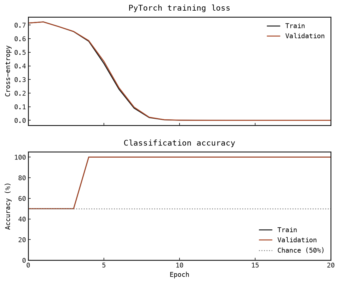
With the supplied settings, both splits reach 100% accuracy during training. Reloaded hybrid weights also classify all 64 test samples correctly. All 64 input weights, all 32 readout weights, and all head weights and biases change. This is an intentionally easy synthetic task.
10. Integration boundaries
The current interface is GraphExecutor, not a lang.to_torch conversion function. It executes the supported compiled graph using PyTorch operations and the snnlab spiking implementation; it does not export a dependency-free network.
Inputs to the executor are named tensors, and its direct result is an ExecutionResult. The wrapper adapts these to your application’s tensor interface. Each call starts with fresh dynamic state unless continuation state is explicitly supplied. Returned continuation state is detached, so gradients do not span separate continued calls.
Declared outputs retain gradients. Exposed diagnostics are detached, and result.numpy() produces detached copies. When training a custom PyTorch head, use tensor outputs directly and declare the features it needs with net.output before compiling the bundle.