Inference
Load the training example's saved network and learned weights, classify fresh spike patterns, and inspect its responses.
Use the network from Training to recognise new spike patterns. The task is the same: decide whether channels 0–1 or channels 2–3 are more active. This time, the network uses the weights it has already learned. It makes predictions without updating them.
The script loads examples/training/network.bundle and examples/training/trained.checkpoint. It generates 64 fresh samples, chooses the class with the higher readout score, and compares those predictions with the known labels.
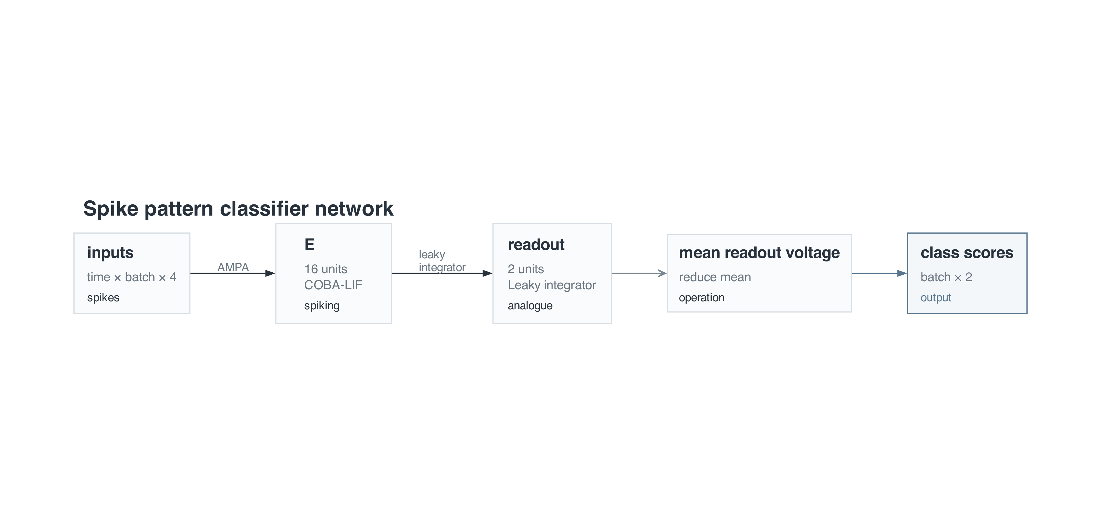
The diagram is generated from the saved bundle. This walkthrough loads that network rather than defining or compiling a new one. Run the Training example first; all inference outputs are saved separately in examples/inference/.
1. Imports and saved artifact paths
import json
from pathlib import Path

import numpy as np
import torch

from snnlab import lang, viz
from snnlab.sim.execution import DenseArrayBinding, ExecutionSpec, infer

OUTPUT_DIR = Path(__file__).resolve().parent
TRAINING_DIR = OUTPUT_DIR.parent / "training"
DT_MS = 0.5
DURATION_MS = 200
HIGH_RATE_HZ = 100
LOW_RATE_HZ = 10
TEST_SAMPLES = 64
DATA_SEED = 20
MODEL_SEED = 17
CLASS_NAMES = ("A", "B")bundle_path = TRAINING_DIR / "network.bundle"
checkpoint_path = TRAINING_DIR / "trained.checkpoint"
for path in (bundle_path, checkpoint_path):
if not path.is_dir():
raise FileNotFoundError(
f"Missing {path}. Run uv run python examples/training/training.py first."
)network.bundle supplies the graph and its declarations. trained.checkpoint supplies the learned w_in and w_out weights. Paths are relative to the script, so running it from another working directory still finds the paired Training example. Missing artifacts produce an error explaining how to generate them.
2. Load the saved network and diagram
bundle = lang.load_bundle(bundle_path)
diagram = lang.diagram(bundle, view="expanded")
viz.render_diagram(
diagram,
OUTPUT_DIR / "network.png",
scale=2,
height_to_width_ratio=None,
canvas_size=(1920, 900),
)lang.load_bundle verifies and loads the saved bundle. Rendering its expanded diagram gives the overview shown above. Graphviz’s dot executable must be on your PATH; on macOS, install it with brew install graphviz.
This loads the network description. The checkpoint field in step 4 tells the executor to load its learned weights before running it.
3. Generate fresh inputs
The dataset helper uses the same rate patterns and ±15% variation as Training. DATA_SEED=20 differs from both the training seed (18) and validation seed (19). Class A is label 0, and class B is label 1.
def make_dataset(samples, seed):
"""Use the training task's patterns with new rate variation and spike draws."""
rng = np.random.default_rng(seed)
labels = np.arange(samples) % 2
rng.shuffle(labels)
patterns = np.array(
[
[HIGH_RATE_HZ, HIGH_RATE_HZ, LOW_RATE_HZ, LOW_RATE_HZ],
[LOW_RATE_HZ, LOW_RATE_HZ, HIGH_RATE_HZ, HIGH_RATE_HZ],
]
)
rates = patterns[labels] * rng.uniform(0.85, 1.15, size=(samples, 4))
probability = rates * DT_MS / 1000
steps = round(DURATION_MS / DT_MS)
spikes = rng.random((steps, samples, 4)) < probability
return torch.tensor(spikes, dtype=torch.float32), torch.tensor(
labels, dtype=torch.long
)input_spikes, labels = make_dataset(TEST_SAMPLES, seed=DATA_SEED)
test_input = DenseArrayBinding(input_id="inputs", value=input_spikes)The DenseArrayBinding matches the saved graph’s input named "inputs". Spikes have (400, 64, 4) axes: time, sample and input channel. Keep the timing and rate settings aligned with Training when modifying this paired example.
Labels are used to assess predictions after inference. They are not passed to infer, which does not need the correct answer to run.
4. Load learned weights and infer
execution = ExecutionSpec(
kind="infer",
bundle=bundle_path,
checkpoint=checkpoint_path,
input_bindings=(test_input,),
seed=MODEL_SEED,
device="cpu",
)
with torch.no_grad():
result = infer(execution)ExecutionSpec.checkpoint loads the Training checkpoint’s named parameters. Inference checks the graph identity and parameter compatibility. It does not restore the optimizer or resume training.
torch.no_grad() prevents gradient tracking. There is no optimizer step or training call. Diagnostics are enabled by default, so the signals exposed in Training are available for the plots: input spikes, E spikes and readout voltages.
5. Retrieve scores and predictions
data = result.numpy()
scores = data.outputs["class_scores"]
predictions = scores.argmax(axis=1)
expected = labels.numpy()
accuracy = float(np.mean(predictions == expected))
print(f"Accuracy on {TEST_SAMPLES} fresh samples: {accuracy:.1%}")result.numpy() returns named NumPy arrays. class_scores has shape (64, 2): one row per sample and one score per class. argmax(axis=1) selects the higher-scoring class. These scores are logits, not probabilities.
Accuracy is the fraction of predictions matching the known labels. With the supplied training configuration and seeds, the saved model classifies all 64 samples correctly. This measures the synthetic task, not performance on real neural recordings.
6. Save predictions and plot responses
predictions_path = OUTPUT_DIR / "predictions.json"
predictions_path.write_text(
json.dumps(
{
"accuracy": accuracy,
"data_seed": DATA_SEED,
"checkpoint": result.metrics["checkpoint"],
"labels": expected.tolist(),
"predictions": predictions.tolist(),
"class_scores": scores.tolist(),
},
indent=2,
)
+ "\n"
)predictions.json records labels, predictions, both scores, accuracy and checkpoint provenance. Provenance identifies the loaded checkpoint and its completed update count.
The plotting code selects one fresh sample from each class. Each column shows its four input spike trains, the sixteen E neurons’ spikes and both readout voltage traces. The three rows share a time axis within each column. The predicted class is determined by mean readout voltage over the whole presentation. Plotting code is included only in the full example.
7. Full example
In a repository checkout, run these commands in order:
uv run python examples/training/training.py
uv run python examples/inference/inference.pyDownload the complete inference script and place it in examples/inference/ alongside the paired examples/training/ directory.
It saves these files beside the inference script:
network.png: diagram generated from Training’s saved bundle.predictions.json: predictions, accuracy and loaded checkpoint provenance.inference.png: responses for one sample from each class.
Rerunning inference replaces its own generated outputs and leaves the Training bundle and checkpoint untouched. It never starts training automatically.
"""Load the training example's saved model and classify fresh spike patterns."""
import json
from pathlib import Path
import matplotlib
matplotlib.use("Agg")
import matplotlib.pyplot as plt
import numpy as np
import torch
from snnlab import lang, viz
from snnlab.sim.execution import DenseArrayBinding, ExecutionSpec, infer
OUTPUT_DIR = Path(__file__).resolve().parent
TRAINING_DIR = OUTPUT_DIR.parent / "training"
DT_MS = 0.5
DURATION_MS = 200
HIGH_RATE_HZ = 100
LOW_RATE_HZ = 10
TEST_SAMPLES = 64
DATA_SEED = 20
MODEL_SEED = 17
CLASS_NAMES = ("A", "B")
def make_dataset(samples, seed):
"""Use the training task's patterns with new rate variation and spike draws."""
rng = np.random.default_rng(seed)
labels = np.arange(samples) % 2
rng.shuffle(labels)
patterns = np.array(
[
[HIGH_RATE_HZ, HIGH_RATE_HZ, LOW_RATE_HZ, LOW_RATE_HZ],
[LOW_RATE_HZ, LOW_RATE_HZ, HIGH_RATE_HZ, HIGH_RATE_HZ],
]
)
rates = patterns[labels] * rng.uniform(0.85, 1.15, size=(samples, 4))
probability = rates * DT_MS / 1000
steps = round(DURATION_MS / DT_MS)
spikes = rng.random((steps, samples, 4)) < probability
return torch.tensor(spikes, dtype=torch.float32), torch.tensor(
labels, dtype=torch.long
)
def main():
# 1. Locate the saved training artifacts.
bundle_path = TRAINING_DIR / "network.bundle"
checkpoint_path = TRAINING_DIR / "trained.checkpoint"
for path in (bundle_path, checkpoint_path):
    if not path.is_dir():
        raise FileNotFoundError(
            f"Missing {path}. Run uv run python examples/training/training.py first."
        )
# 2. Load the saved network and generate its diagram.
bundle = lang.load_bundle(bundle_path)
diagram = lang.diagram(bundle, view="expanded")
viz.render_diagram(
    diagram,
    OUTPUT_DIR / "network.png",
    scale=2,
    height_to_width_ratio=None,
    canvas_size=(1920, 900),
)
# 3. Generate fresh inputs and bind them to the saved network.
input_spikes, labels = make_dataset(TEST_SAMPLES, seed=DATA_SEED)
test_input = DenseArrayBinding(input_id="inputs", value=input_spikes)
# 4. Load learned weights and run inference.
execution = ExecutionSpec(
    kind="infer",
    bundle=bundle_path,
    checkpoint=checkpoint_path,
    input_bindings=(test_input,),
    seed=MODEL_SEED,
    device="cpu",
)
with torch.no_grad():
    result = infer(execution)
# 5. Retrieve scores, choose classes and measure accuracy.
data = result.numpy()
scores = data.outputs["class_scores"]
predictions = scores.argmax(axis=1)
expected = labels.numpy()
accuracy = float(np.mean(predictions == expected))
print(f"Accuracy on {TEST_SAMPLES} fresh samples: {accuracy:.1%}")
# 6. Save predictions and checkpoint provenance.
predictions_path = OUTPUT_DIR / "predictions.json"
predictions_path.write_text(
    json.dumps(
        {
            "accuracy": accuracy,
            "data_seed": DATA_SEED,
            "checkpoint": result.metrics["checkpoint"],
            "labels": expected.tolist(),
            "predictions": predictions.tolist(),
            "class_scores": scores.tolist(),
        },
        indent=2,
    )
    + "\n"
)
# Plot one fresh sample from each class.
grid = viz.FigureGrid(
rows=3,
columns=2,
bounds=(0.09, 0.09, 0.86, 0.85),
row_gap=0.08,
column_gap=0.11,
)
for column in range(2):
for row, name in enumerate(("inputs", "spikes", "readout")):
grid.place(f"{name}_{column}", row=row, column=column)
figure = grid.figure(figsize=(11, 8), dpi=150)
for column, class_name in enumerate(CLASS_NAMES):
sample = int(np.flatnonzero(expected == column)[0])
sample_data = result.numpy(batch=sample)
time_ms = sample_data.time_ms
assert time_ms is not None
input_axis = grid.add_axes(figure, f"inputs_{column}")
spike_axis = grid.add_axes(figure, f"spikes_{column}", sharex=input_axis)
readout_axis = grid.add_axes(figure, f"readout_{column}", sharex=input_axis)
for axis, values, ylabel in (
(input_axis, sample_data.diagnostics["input_spikes"], "Input channel"),
(spike_axis, sample_data.diagnostics["e_spikes"], "E cell"),
):
steps, cells = np.nonzero(values)
axis.scatter(time_ms[steps], cells, marker="|", s=24, color="#1a1a1a")
axis.set_ylim(-0.5, values.shape[1] - 0.5)
axis.set_ylabel(ylabel)
axis.tick_params(labelbottom=False)
input_axis.set_yticks(range(4))
spike_axis.set_yticks((0, 5, 10, 15))
predicted_name = CLASS_NAMES[predictions[sample]]
input_axis.set_title(
f"True class {class_name}; predicted {predicted_name}", pad=10
)
voltages = sample_data.diagnostics["readout_voltage"]
for index, color in enumerate(("#1a1a1a", "#a74727")):
readout_axis.plot(
time_ms,
voltages[:, index],
color=color,
label=f"Class {CLASS_NAMES[index]}",
linewidth=1,
)
readout_axis.set_ylabel("Readout voltage (mV)")
readout_axis.set_xlabel("Time (ms)")
readout_axis.set_xlim(0, DURATION_MS)
readout_axis.legend(frameon=False, fontsize=9)
figure_path = OUTPUT_DIR / "inference.png"
figure.savefig(figure_path, bbox_inches="tight")
plt.close(figure)
print(f"Loaded {checkpoint_path}")
print(f"Saved {predictions_path}")
print(f"Saved {figure_path}")
if __name__ == "__main__":
main()8. Inference responses
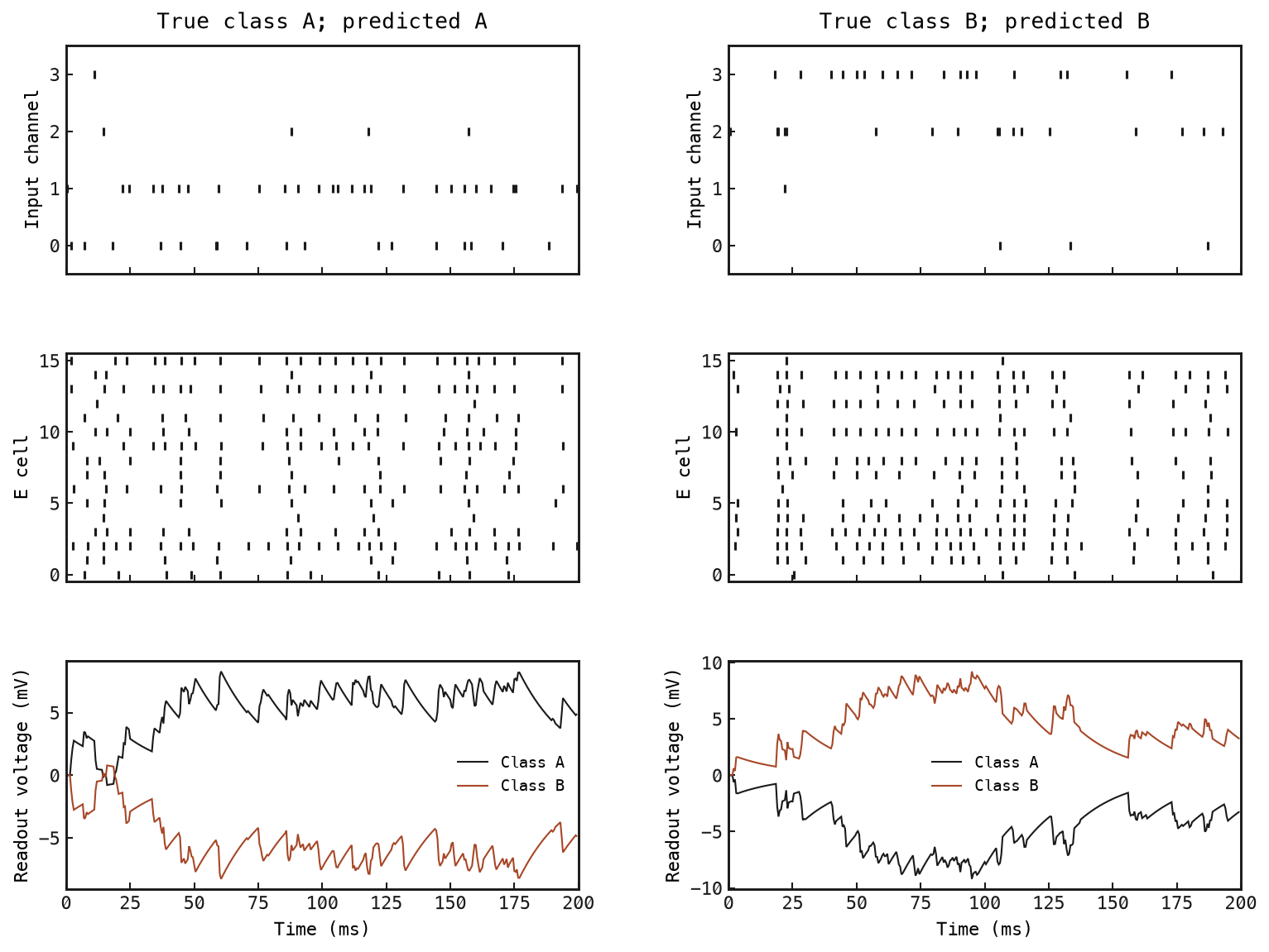
Class A samples drive channels 0–1 more strongly, while class B samples drive channels 2–3 more strongly. The learned network produces a higher mean readout voltage for the matching class.
Change DATA_SEED and rerun inference to try new spike draws with the same saved weights. Changing the seed does not retrain the network.