Quickstart
Define inputs, build an excitatory layer, simulate it and plot the results.
Run one layer of 16 excitatory neurons on CPU, driven by 4 independent Poisson input channels at 80 Hz. The walkthrough follows the script in order. Start by installing snnlab.
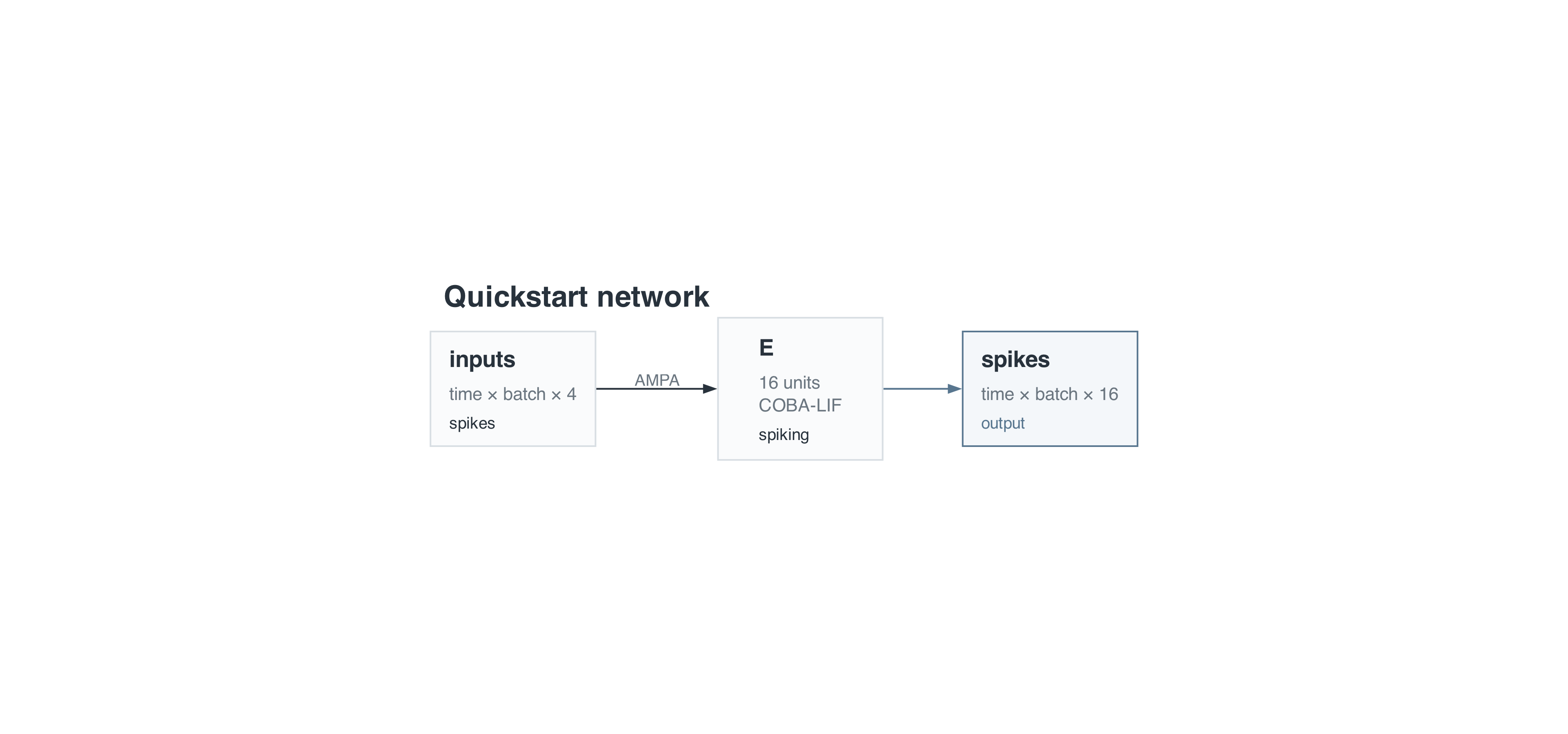
Each input channel connects to every E neuron. The simulation shows how the incoming spikes drive the neurons to fire; the plots below show the inputs, E spikes and membrane voltage.
1. Imports and network definition
Import the authoring and execution APIs and choose the timing and seed:
from snnlab import lang, viz
from snnlab.sim.execution import ExecutionSpec, PoissonInputBinding, simulate

DT_MS = 0.1
DURATION_MS = 300
INPUT_RATE_HZ = 80
SEED = 17
Create the network container with a 0.1 ms timestep:
net = lang.Network("quickstart", dt=DT_MS * lang.ms)2. Define inputs and their binding
Declare the input and choose its Poisson stimulus:
inputs = net.input(
    "inputs", shape=("time", "batch", 4), signal_type="spikes", unit="spike"
)
poisson_input = PoissonInputBinding(
    input_id="inputs",
    steps_count=round(DURATION_MS / DT_MS),
    rates_hz=(INPUT_RATE_HZ,),
    seed=SEED,
)
net.input declares the input contract: spike values with (time, batch, channels) axes and 4 channels. It returns a signal you can connect to neurons. PoissonInputBinding describes how to generate the input for this run. Its input_id="inputs" matches the graph input’s name.
The binding supplies 3,000 time steps and one batch item. At a timestep of 0.1 ms, that is 300 ms. Each input channel is sampled independently at 80 Hz.
Other input bindings are available for different input sources:
DenseArrayBinding: custom input tensors, including NumPy arrays converted withtorch.as_tensor(array).EventStreamBinding: sparse spike events specified by time-step, batch and channel coordinates.DatasetSnapshotBinding: inputs from a saved NPZ dataset, with an encoder and optional training targets.
All are supplied through ExecutionSpec.input_bindings. See the input binding reference for their fields and compatibility rules.
3. Define the network
Create the excitatory layer and connect the input to it:
cells = net.population("E", size=16, neuron=lang.COBA_LIF(tau_mem=20 * lang.ms))
# Connect all 4 input channels to all 16 E cells using 64 weights.
net.connect(
    inputs,
    cells.excitatory,
    name="input_to_E",
    synapse=lang.AMPA(tau=2 * lang.ms),
    weight=lang.Uniform(0.1, 0.5),
    constraint=lang.NonNegative(),
)
COBA_LIF describes conductance-based leaky integrate-and-fire neurons; tau_mem sets their 20 ms membrane time constant. The AMPA projection delivers excitatory conductance with a 2 ms decay time. Its weight initializer samples values uniformly between 0.1 and 0.5 in the projection’s conductance units, microsiemens. NonNegative constrains weights to non-negative values.
Each of the 4 input channels connects to every one of the 16 E cells. net.connect automatically sizes the weight matrix from the source channel count and target neuron count. This creates 64 weights, arranged in a (16, 4) matrix in the compiled graph: one row per E cell and one column per input channel. Each cell receives its own weighted combination of the same four spike trains, so input channels and neurons do not need matching counts.
Uniform(0.1, 0.5) initializes all 64 weights independently. The graph executor divides projection weights by the number of input channels (4 here); see the weight reference for this normalization. Different weights give cells different responses.
See Network.connect for all connection arguments and available options:
- Synapses: AMPA, GABA and leaky-integrator projections, plus the current backend support limits.
- Weights: constant, zero, uniform and normal initializers, or an existing parameter.
- Constraints: no constraint or
NonNegative.
4. Choose outputs and expose diagnostics
# The official network output: spikes.
net.output("spikes", cells.spikes)
# Expose input spikes and membrane voltage for diagnostics.
net.expose(inputs, name="input_spikes")
net.expose(cells.voltage, name="e_voltage")
net.output declares the official network output. Here, excitatory spikes appear in result.outputs["spikes"], even when diagnostics are disabled.
net.expose exposes a diagnostic signal. Exposed signals are returned by default, so input spikes appear in result.diagnostics["input_spikes"] and membrane voltage appears in result.diagnostics["e_voltage"]. Set diagnostics=False in ExecutionSpec to disable them.
5. Bundle the network
Compile the network into an in-memory bundle:
bundle = lang.compile(net, target="tools/snnsim")
diagram = lang.diagram(bundle, view="expanded")
viz.render_diagram(
    diagram,
    OUTPUT_DIR / "network.png",
    scale=2,
    height_to_width_ratio=None,
    canvas_size=(1920, 900),
)
Compilation validates the network. The script passes bundle.graph directly to execution.
You can also save the bundle for later use:
bundle_path = bundle.write("quickstart.bundle")To run the saved bundle, pass bundle=bundle_path to ExecutionSpec in place of graph=bundle.graph. Choose either the in-memory graph or the saved bundle route.
6. Configure execution and simulate
execution = ExecutionSpec(
    kind="simulate",
    graph=bundle.graph,
    input_bindings=(poisson_input,),
    seed=SEED,
    device="cpu",
)
result = simulate(execution)
The graph executor is the default. input_bindings supplies the Poisson stimulus by name, device="cpu" selects CPU execution, and exposed diagnostics are returned by default. simulate executes the request and returns the result. See the ExecutionSpec reference for every setting.
7. Retrieve outputs and prepare plots
data = result.numpy(batch=0)
input_spikes = data.diagnostics["input_spikes"]
spikes = data.outputs["spikes"]
voltages = data.diagnostics["e_voltage"]
time_ms = data.time_ms
assert time_ms is not None
spikes comes from the official network output; input_spikes and voltages come from the exposed diagnostics. result.numpy(batch=0) converts them to independent NumPy arrays and selects the first batch item using each signal’s declared axes. data.time_ms supplies the time axis in milliseconds using the actual simulation timestep. The original result retains its tensors. See the NumPy result reference for details.
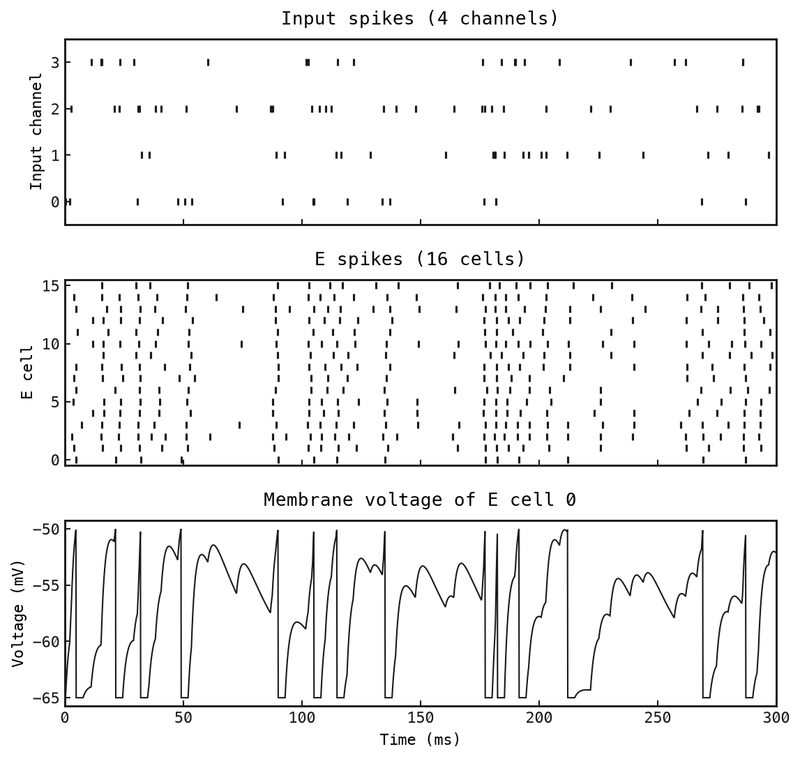
The plotting step uses snnlab.viz.FigureGrid and Matplotlib to save one figure with three rows: input spikes, E spikes and E cell 0’s membrane voltage. All rows share the same time axis. Its implementation is included in the full script below.
8. Full example
Save the complete script as examples/quickstart/quickstart.py in your project. In a repository checkout, it is already there.
uv run python examples/quickstart/quickstart.pyIt writes network.png and quickstart.png beside the script, regardless of your working directory. Rerunning replaces those files. Rendering the network diagram requires Graphviz’s dot executable on your PATH; on macOS, install it with brew install graphviz. No dataset download is needed.
"""Simulate a single excitatory layer and save one figure beside this script."""

from pathlib import Path

import matplotlib

matplotlib.use("Agg")
import matplotlib.pyplot as plt
import numpy as np

from snnlab import lang, viz
from snnlab.sim.execution import ExecutionSpec, PoissonInputBinding, simulate

OUTPUT_DIR = Path(__file__).resolve().parent
DT_MS = 0.1
DURATION_MS = 300
INPUT_RATE_HZ = 80
SEED = 17


def main():
    # 1. Create the network.
    net = lang.Network("quickstart", dt=DT_MS * lang.ms)
    # 2. Define the input and its stimulus binding.
    inputs = net.input(
        "inputs", shape=("time", "batch", 4), signal_type="spikes", unit="spike"
    )
    poisson_input = PoissonInputBinding(
        input_id="inputs",
        steps_count=round(DURATION_MS / DT_MS),
        rates_hz=(INPUT_RATE_HZ,),
        seed=SEED,
    )
    # 3. Define the excitatory layer and its input projection.
    cells = net.population("E", size=16, neuron=lang.COBA_LIF(tau_mem=20 * lang.ms))
    # Connect all 4 input channels to all 16 E cells using 64 weights.
    net.connect(
        inputs,
        cells.excitatory,
        name="input_to_E",
        synapse=lang.AMPA(tau=2 * lang.ms),
        weight=lang.Uniform(0.1, 0.5),
        constraint=lang.NonNegative(),
    )
    # 4. Choose outputs and exposed diagnostics.
    # The official network output: spikes.
    net.output("spikes", cells.spikes)
    # Expose input spikes and membrane voltage for diagnostics.
    net.expose(inputs, name="input_spikes")
    net.expose(cells.voltage, name="e_voltage")
    # 5. Compile the network into a bundle.
    bundle = lang.compile(net, target="tools/snnsim")
    diagram = lang.diagram(bundle, view="expanded")
    viz.render_diagram(
        diagram,
        OUTPUT_DIR / "network.png",
        scale=2,
        height_to_width_ratio=None,
        canvas_size=(1920, 900),
    )

    # 6. Describe the execution and simulate.
    execution = ExecutionSpec(
        kind="simulate",
        graph=bundle.graph,
        input_bindings=(poisson_input,),
        seed=SEED,
        device="cpu",
    )
    result = simulate(execution)
    # 7. Retrieve named results and select the first (only) batch item.
    data = result.numpy(batch=0)
    input_spikes = data.diagnostics["input_spikes"]
    spikes = data.outputs["spikes"]
    voltages = data.diagnostics["e_voltage"]
    time_ms = data.time_ms
    assert time_ms is not None

    # Plot the results with snnlab.viz and Matplotlib.
    grid = viz.FigureGrid(
        rows=3, columns=1, bounds=(0.12, 0.09, 0.85, 0.85), row_gap=0.07
    )
    grid.place("inputs", row=0, column=0)
    grid.place("spikes", row=1, column=0)
    grid.place("voltage", row=2, column=0)
    figure = grid.figure(figsize=(8, 7.5), dpi=150)
    input_axis = grid.add_axes(figure, "inputs")
    spike_axis = grid.add_axes(figure, "spikes", sharex=input_axis)
    voltage_axis = grid.add_axes(figure, "voltage", sharex=input_axis)

    for axis, values, title, label in (
        (input_axis, input_spikes, "Input spikes (4 channels)", "Input channel"),
        (spike_axis, spikes, "E spikes (16 cells)", "E cell"),
    ):
        steps, cell_ids = np.nonzero(values)
        axis.scatter(time_ms[steps], cell_ids, marker="|", s=24, color="#1a1a1a")
        axis.set_ylim(-0.5, values.shape[1] - 0.5)
        axis.set_yticks(
            np.linspace(0, values.shape[1] - 1, min(values.shape[1], 4), dtype=int)
        )
        axis.set_ylabel(label)
        axis.set_title(title, pad=10)
        axis.tick_params(labelbottom=False)

    voltage_axis.plot(time_ms, voltages[:, 0], color="#1a1a1a", linewidth=1)
    voltage_axis.set_ylabel("Voltage (mV)")
    voltage_axis.set_title("Membrane voltage of E cell 0", pad=10)
    voltage_axis.set_xlabel("Time (ms)")
    voltage_axis.set_xlim(0, DURATION_MS)
    path = OUTPUT_DIR / "quickstart.png"
    figure.savefig(path, bbox_inches="tight")
    plt.close(figure)
    print(f"Saved {path}")

    counts = spikes.sum(axis=0)
    print(f"Total spikes: {int(counts.sum())}")
    print(f"Spikes per cell: {counts.astype(int).tolist()}")


if __name__ == "__main__":
    main()
9. Plots
The three rows share a time axis, making it easy to compare the stimulus with the excitatory layer’s response:
- Input spikes: each mark is an incoming spike on one of the 4 Poisson input channels.
- E spikes: each mark is an emitted spike from one of the 16 excitatory cells.
- Voltage: E cell 0’s membrane voltage in millivolts. Input raises it toward threshold; after a spike, the voltage resets.
Change INPUT_RATE_HZ from 80 to 40, rerun, and compare the input and response while keeping the other settings fixed.